Shromona Ganguly and Deepa S. Raj* Received on: August 31,2020
Accepted on: December 17, 2020 The study examines determinants of default in education loans in Tamil Nadu, a state with significant presence in education loan disbursal in the country. It uses account level data of over two lakh borrowers from two public sector banks and one private sector bank in an attempt to identify significant predictors of default. Empirical analysis suggests that loan accounts with higher interest rate and of lower duration have higher default probability while loans extended to accounts with Aadhar information, collateral backing or some subsidy element have lower risk of default. JEL Codes: I22, I25, I28 Keywords: Education loan, non-performing assets, default risk, interest subsidy Introduction Education loans provide institutional funding required to harness and empower the human capital in a country, given the financial constraints faced by the public sector and individuals in meeting the rising cost of education. With governments, both at the national and sub-national levels, focused on providing universal primary education, the growing needs of a young nation like India in the sphere of higher education are increasingly being fulfilled by the private sector, although public sector institutions continue to play a significant role. Education loan portfolio forms only a small fraction of retail loan portfolio of all commercial banks in India (3.3 per cent) but it bears special significance in terms of skill formation required for enhancing productivity and efficiency in an economy. It is in this light that the sharp increase in non-performing assets (NPA) in education loans extended by commercial banks in India in recent years is a matter of concern, as it could hamper the growth of bank credit for higher education in the country. Though economic theory focuses more on managing common pool resources (Ostrom, 2010), a special feature of higher education is that it suffers from the problem of “reverse tragedy of commons” (Piirainen et al., 2018; Mor, 2019) where the benefit that accrues to the society for imparting skill and knowledge surpasses the private cost associated with acquiring such skill and thereby results in underproduction of higher education in relation to the socially optimal or desirable level. Surmounting this problem requires huge investment in the education sector, which is challenging for developing economies, given their relatively low per capita income and high public debt. According to the United Nation’s human development data1, gross enrolment ratio in tertiary education2 during 2014-19 was 28 per cent for India, which was lower than the average of 33 per cent for developing countries and the world average of 39 per cent. Given that higher education helps in attaining sustainable livelihoods, it is important to bridge the resource gap for meritorious students with limited means, particularly in countries where private market for education loans is underdeveloped. Worldwide, countries adopt various policies to address the issue of missing markets in the context of financing education which can be broadly divided into two types - government aid-based measures and private loans (Wegmann et al., 2003; Barr, 2004; Field 2009). India had initially envisaged a policy of state-led development of higher education, and the Education Commission (1964-66) chaired by D. S. Kothari was emphatic in its recommendations that most of the responsibility for the support of education should be from government funds and not from the private sector. However, the same has undergone a change overtime, with the number of private institutions growing rapidly since the mid-eighties (Tilak, 2007). Nevertheless, several policy measures taken over the years by the Government of India include provision of interest rate subsidies for education loans, inclusion of education loans up to certain prescribed limit within priority sector definition and establishment of credit guarantee fund for provision of guarantee cover against education loan default. Despite these measures, the number of accounts under priority sector education loan category has been declining since 2017-18. The vast literature on issues associated with student loan market mainly focus on advanced economies, especially the US (Wilms et al., 1987; Volkwein and Szelest, 1995; Knapp and Seaks, 1992; Flint 1994), where the outstanding student loan is almost 7.5 per cent of the country’s GDP in 2019 and the rising default rate in student loan remains a cause for concern for lenders as well as policymakers (Ben, 2018; Forbes, 2019). Studies on student loan default in these advanced economies often lack consensus on the common factors responsible for default, though it is generally found that borrowers’ income level, gender, ethnic group, student performance and choice of education courses are significant predictors of default probability (Stockham and Hesseldenz,1979; Herr and Burt, 2005), along with spatial and macro-economic factors such as growth and employment scenario (Dynarski, 1994; Monteverde, 2000; Hillman, 2014). In contrast, studies which discuss problems associated with student loan market in developing countries are sparse. Further, so far there have been very few attempts to empirically analyse issues pertaining to education loan in India, particularly those relating to default in these loans, mainly due to lack of availability of detailed data. In this context, this study seeks to augment the existing literature on education loan default in developing countries. It analyses the nature of education loan NPAs in Tamil Nadu, which not only features amongst the states with high education loans as well as NPAs in the same but is also a state with a significant presence of private institutions, especially in professional and technical education.3 In the absence of sufficient studies on student loan default in developing economies, this paper does not propose a testable hypothesis. Instead, the study explores the rich account level data on education loan extended by two large public sector banks (PSBs) and one private sector bank (PVB) headquartered in the southern region to borrowers in the state in an attempt to understand the major determinants of default in the education loan segment. The data pertain to the education loan portfolio of the selected banks as at end-March 2019 and are sourced from their respective management information systems. The study also presents the main results of a survey conducted among banks in the state to obtain the lender’s perspective of the problems of education loan default. Thus, to the best of our knowledge, this is the first state specific study in the Indian context, which analyses education loan default with the help of a large dataset representing both public sector and private sector banks. The rest of the paper is structured as follows: Section II provides an overview of education loan schemes in India as well as other countries and the recent trends in education loan in India and Tamil Nadu, including NPAs in this segment. Section III discusses the theoretical underpinning as well as empirical findings related to education loan default as documented in literature. Section IV provides a descriptive analysis of the data obtained from select banks in the state, followed by empirical framework adopted in the paper. Section V presents the main results of the empirical exercise and implications thereof. Section VI sets out the findings of a questionnaire-based survey relating to the education loan portfolio of lending banks in Tamil Nadu conducted in July 2020. Section VII concludes the study by summarising the major findings, policy implications, some limitations of the present study and scope for future research. Section II
Overview of Education Loans II.1 Types of Education Loans: Cross Country Comparison Worldwide, there are various types of education loans available to the students which can be broadly classified into three categories (Jayadev, 2017). In the conventional mortgage type loans (CMLs), the loan repayment period, monthly schedule of repayments and the interest rate are determined by the loan agreement, irrespective of the income of the borrower at the completion of the course. CML is popular in China and Japan. On the contrary, income contingent loans (ICLs) link the amount to be repaid in each installment with the earning capacity of the borrower. Such schemes are popular in Australia and United Kingdom. A third category of educational loans, popularly known as fixed schedule income contingent loans (FSICs), fix the minimum amount of repayment per installment, and additional amount to be repaid depends on the earning ability of the graduate. FSIC is popular in the US, South Korea and Norway. Each of these schemes has its own advantages as well as disadvantages. In the case of CML, both the debt burden and the repayment period are known to the borrower as well as to the banks, irrespective of any contingency. However, this often results in banks not tracking the employment and income of the borrowers after the completion of the course. In many cases, since the initial income of the borrower after the completion of the course would be substantially low, this may often lead to high debt repayment burden in the initial years and high delinquency rate. Under the ICL, the installment amount is a proportion of total income earned by the borrower. It is a better mechanism of consumption smoothening as it allows the graduates to accelerate their repayment if their incomes are high or repay a lower amount if their initial incomes are low. ICL is implemented by directly deducting the required amount from the borrowers’ salary by the tax authorities in many countries. ICLs are explicitly designed to reduce the repayment burden of the borrowers and in countries with efficient tax collection offices, this method is proven to be more cost efficient than any other instrument of financing higher education. Further, education loans are often subject to market failure as in most cases such loans are not backed by collaterals. As a result, there is under-allocation of such loans as compared with the social optimal level. Presence of government guarantee could solve this problem although the same comes with other issues and problems. ICL is often proposed as an alternative to the government guarantee in education loans. Initially adopted in Sweden as an alternative to government subsidised loan programme, ICL later became popular in New Zealand, Chile, South Africa, the UK and the US. ICL varies across these countries in terms of its structure, design and implementation. The most common forms of these loans are ICL with risk pooling, ICL with risk sharing, graduate taxes and human capital contracts. II.2 Types of Education Loan in India The education loan schemes offered by banks in India are in the nature of CMLs, which can be further classified into the different categories on the basis of student borrower characteristics and institutions they seek admissions to/study in. Most banks offer a scheme for education loan as per the Indian Banks’ Association (IBA) model education loan scheme to students pursuing higher studies in India and abroad. As per this model loan scheme, education loans up to ₹4 lakh do not require any collateral to be provided by the borrower, education loans up to ₹7.5 lakh can be obtained with collateral in the form of suitable third-party guarantee, while education loans above ₹7.5 lakh require tangible collateral. In all the above cases, co-obligation of parents is necessary. The second category of education loans are sanctioned to those students who obtain admissions to colleges/universities through management quota, provided they satisfy the minimum marks criteria in the preceding examination. The third category of education loans includes schemes for needy students for pursuing vocation education courses run by industrial training institutes (ITIs), polytechnics, training partners affiliated to National Skill Development Corporation (NSDC)/sector skill councils, state skill mission/corporation, preferably leading to a certificate/diploma/degree issued by such organisation as per National Skill Qualification Framework (NSQF) and any other institutions recognized by either the central or state education boards or university. The fourth category of scheme specifically caters to the requirement of students studying in premier institutions like IITs/IIMs/NITs/IISc or courses abroad, with demand for a higher quantum of loan amount. All education loans of up to ₹10 lakh (enhanced to ₹20 lakh in September 2020) have been included within the priority sector definition by the Reserve Bank of India. Under most of these schemes, moratorium period consists of the course period plus six months to one year, and there are nil/negligible processing fees for schemes with high value education loans. The interest rate under the various schemes consists of a markup of 2-3 per cent above the marginal cost of funds based lending rate (MCLR)/external benchmark4, based on the reputation of the course/institutions. The repayment period is in the range of 10-15 years. II.3 Education Loan in Tamil Nadu: State Profile and Institutional Setup In India, around 90 per cent of education loans are disbursed by the PSBs, while PVBs and regional rural banks (RRBs) account for around 7 per cent and 3 per cent of total education loan outstanding, respectively, as at end- March 20205. During the same year, PSBs accounted around 94 per cent of total education loan disbursement in Tamil Nadu while PVBs accounted for 6 per cent. Out of total education loan outstanding in the state as at end-March 2020, semi-urban area accounted for 38 per cent, followed by rural area (26 per cent), metropolitan region (21 per cent) and urban area (15 per cent). Bank-wise data available for Tamil Nadu6 shows that education loan sanctioned during 2019-20 was the highest for State Bank of India (SBI) among all scheduled commercial banks (18.4 per cent), followed by Canara Bank (17.0 per cent) and Indian Bank (11.4 per cent). Among the PVBs, education loan sanctioned by Axis Bank was the highest (4.2 per cent), followed by Tamil Nadu Mercantile Bank (3.2 per cent). In terms of number of education loan accounts, Canara Bank topped the list, indicating smaller loan size than SBI (Appendix Table 1). During this decade, growth in education loan portfolio was on a decelerating trend till 2013-14, both in Tamil Nadu and at all-India level, before reviving to double digits in 2014-15, only to moderate in the subsequent years. Education loan growth for Tamil Nadu turned negative in 2018-19 although the rate of decline moderated in 2019-20 (Chart 1a). While the growth in PSB advances mirrored that in overall education loans by all commercial banks, growth in advances by PVBs increased sharply in 2018-19 but turned negative in 2019-20 (Chart 1b). The number of applications received by banks in the state for education loan has also declined since 2018-19, indicating reduced demand for the same. This could be ascribed to technical courses losing their sheen in the face of declining absorptive capacity of the job market, on the one hand and remunerations incommensurate with the high cost of such education, on the other. Further, uncertainty stemming from the prevailing COVID-19 pandemic situation has also led to a sharp fall in applications for education loan in the state by 54.3 per cent in H1:2020-21 over the comparable period of the previous year7. Tamil Nadu’s predominance in education loans extended by banks can be partly attributed to the large presence of private educational institutions in the state. As per All India Higher Education Report 2018-19, Tamil Nadu’s gross enrolment ratio at 49 per cent was one of the highest among Indian states. Private unaided institutions in Tamil Nadu accounted for 76.5 per cent of the total number of colleges and 60 per cent of total college enrolment in the state as compared to an all-India average of 64 per cent and 45.2 per cent, respectively. The share of Tamil Nadu in terms of student enrolment in various standalone professional institutions such as polytechnic, hotel management, primary teachers training, nursing and paramedical in the country was around 17 per cent, with the state housing the highest number of polytechnic institutions in India (Table 1). 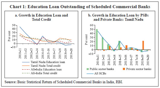
| Table 1: Student Enrolment in Standalone Institutions in Tamil Nadu – 2018-19 | | | Poly- technic | Post Graduate Diploma in Manage- ment | Nursing | Teacher's training | Paramedical | Hotel Manage- ment and Catering | Total | | Number of Institutions | | Tamil Nadu | 496 | 9 | 111 | 292 | - | 2 | 910 | | All-India | 3,440 | 291 | 3,039 | 3,759 | 70 | 26 | 10,625 | | Student Enrolment | | Tamil Nadu | 3,34,180 | 483 | 9,003 | 7,863 | - | 3,53,716 | 7,05,245 | | All-India | 15,13,684 | 50,368 | 2,81,868 | 2,72,599 | 6,801 | 21,47,584 | 42,72,904 | | Source: All-India Survey on Higher Education, 2018-19, Ministry of Human Resource Development, Government of India. | II.4 Subsidy for Education Loans To the students availing education loan, Government of India extends support in the form of a central sector interest subsidy (CSIS) scheme, whereby full interest subsidy is provided during the moratorium period8 on model education loans up to ₹7.5 lakh without collateral security and thirdparty guarantee, for pursuing technical/professional courses in India. Students whose annual gross parental/family income is up to ₹4.5 lakh are eligible for benefits under the scheme. Under the Padho Pardesh scheme, Government of India also provides interest subsidy on education loan availed by meritorious students belonging to economically weaker sections of minority communities for approved post-graduation/doctoral courses offered abroad. Additionally, Government of India, through the National Credit Guarantee Trustee Company (NCGTC), has established a Credit Guarantee Fund for Educational loans (CGFEL) in 2015 to provide guarantee cover of up to 75 per cent against default in uncollateralised educational loan of up to ₹7.5 lakh extended by a registered lender at a rate of interest which is not higher than 2 per cent above the base rate/marginal cost of funds based lending rate (MCLR). Cumulative sanction amount covered under CGFEL was ₹12,121.45 crore as at end-March 2019, with the southern region accounting for 50 per cent of the guarantees to 3.65 lakh accounts given by NCGTC.9 II.5 NPAs in Education Loan While southern states account for the largest proportion of education loans by PSBs, they also dominate in terms of number of accounts turning into NPAs as well as NPA amount outstanding (Chart 2). As at end September 2017, the share of Tamil Nadu in total NPAs in the education loan segment in India was the highest among the Indian states both in terms of number of accounts (50 per cent), and in terms of amount outstanding (42 per cent).
NPA ratio in education loan under the priority sector increased sharply from 9.1 per cent at end-March 2013 to 13.3 per cent at end-March 2016 in Tamil Nadu. The one-time settlement scheme of education loan introduced during 2016-17 led to some moderation, but it rose sharply in the following year and stood at 22.3 per cent as of end-March 2020 (Chart 3). Section III
Education Loan: Theories and Empirics from Literature A vast body of literature deals with the problems associated with designing education loan schemes, in particular, and student debt burden as well as loan default, in general. Most of these studies relate to developed economies, with very few focusing on developing economies, possibly because student loan segment in these countries is still very small in comparison to the burgeoning student loan market of some advanced economies. In the US, the total size of student loan market had surpassed total credit card outstanding for the first time in 2010 and has been growing rapidly since then (Avery and Turner, 2012). Latest data place the outstanding student loan debt in the US at US $1.56 trillion from around 45 million borrowers.10 The empirical literature on education loan deals with several associated issues such as cross country comparison across various higher education loan schemes, cohort analysis, optimal indebtedness and loan repayment burdens of students (Chapman and Lounkaew, 2015; Andruska et al., 2014; Hillman, 2015a, 2015b; Looney and Yannelis, 2015). There is a well-established literature on the subject matter dealt in the present paper i.e., borrower level characteristics and default rate, most of which is in the context of the US (Wilms et al., 1987; Volkwein and Szelest, 1995; Knapp and Seaks, 1992). Flint (1994) analyses students’ pre-college characteristics associated with loan default rate, using data of borrowers who obtained the Stafford loan11 in the US in 1990. The empirical analysis of the paper finds that though students’ grade point average is statistically significant, enrolment choices, amount borrowed, number of loans and reasons for leaving the college are not statistically significant in the context of default. Using data from the National Postsecondary Student Aid Study, Dynarski (1994) finds that low socioeconomic status of borrowers, incomplete or poor educational attainment and low earnings after completion of school were the major determinants of default in education loan. The paper, thus, concludes that efforts to reduce default rates are likely to be felt most significantly by students from disadvantaged backgrounds who were the major recipients of student aid. In the context of developing countries, the magnitude of government spending on education, especially higher education, remains a crucial public policy debate (Birdsall, 1996; Mor, 2019), along with the social implications of subsidy and the resulting adverse selection in the student loan market (Ionescu and Simpson, 2016). In the Indian context, Chandrasekhar et al. (2016) use NSSO’s Survey data on Social Consumption in India (2014) and find that there is binding credit constraint among poorer households in India in availing higher education. However, there are very few studies that focus on the relationship between borrower level characteristics and loan default rate in developing countries. One such study for India which is pertinent for the present paper is Bandyopadhyay (2016). This study empirically investigates the granular level risk of education loan using a cross section of data from 5000 borrowers obtained from four major PSBs in India. The findings suggest that education loan defaults are mainly influenced by security, borrower margin, and repayment periods. The presence of guarantor or co-borrower and collateral significantly reduce default loss rates. The socioeconomic characteristics of borrowers and their regional locations also act as important factors associated with education loan defaults. The results suggest that banks can adopt better risk mitigation and pricing strategies to resolve the issue of bad debt in the education loan portfolio by segmenting borrowers on the basis of probability of default and loss given default in a multidimensional scale. Extending the research in the Indian context, the present study explores the crucial factors associated with education loan default in Tamil Nadu. This study uses a detailed account-level lending data of over two lakh borrowers in the state from three commercial banks headquartered in the southern region as compared to a smaller sample of 5000 borrowers by Bandyopadhyay (2016). Since the southern region, particularly Tamil Nadu, has a dominant presence in education loan market in India, focusing only on the NPAs in education loans in the state throws up some interesting insights which may not have been discovered with the use of diverse all-India data. Further, unlike the study by Bandyopadhyay (2016) which was confined only to PSBs, this study covers two PSBs and one PVB, thereby facilitating a comparison between the two categories of banks by ownership. More specifically, use of micro level data allows us to investigate the spatial, borrower, scheme and course specific attributes associated with higher default probability in education loan segment. Findings of the paper have important policy implications in terms of risk identification in education loan segment. With a view to capture the lenders’ perspective in extending education loan, the paper also includes the results of a questionnaire-based survey of banks in Tamil Nadu. Section IV
Data and Methodology IV.1 Data The paper uses detailed account level information pertaining to March 2019 on socioeconomic characteristics of borrowers along with spatial and other relevant facts obtained from two large PSBs and one PVB operating in Tamil Nadu. Account level information is available for location (branch, district and population group indicating whether the branch is located in urban/semi-urban/rural/metropolitan area of the state), borrowers’ identity (gender, income group, course of study, institution name) and lending parameters (scheme name, interest rate, amount, repayment period, availability of collateral, subsidy status, amount outstanding and NPA status), along with education loan scheme details for each account. Though the same set of information was sought from the three banks, each bank reported the information as per its own format. This is particularly true for fields like education course details, institution details and income group of the borrower. Due to differences in data format, regression results are reported separately for each bank in the following sections. Further, each bank is treated as a separate entity of analysis as it varies significantly from the others in the sample in terms of spatial presence, products offered, clientele and lending practices. For the sake of maintaining anonymity, the analysis in the paper does not name the selected banks. IV.2 Descriptive Statistics Table 2 provides some important statistics related to education loan portfolio of banks in the sample as well as highlights some differences between education loan portfolio of the selected PSBs and PVB. It is found that in all three banks, male borrowers accounted for around two-thirds of the total education loan portfolio, on an average. In terms of spatial dimension, while all three banks had a sizeable share of semi-urban area in the education loan portfolio, the two PSBs had a significantly higher proportion of education loan from rural area and a fairly low proportion of education loan from metropolitan area as compared to the PVB. Significant difference is also observed in the proportion of education loan accounts eligible for subsidy, with the two PSBs having a significantly higher ratio of 61 per cent (Bank A) and 76 per cent (Bank B) as against the PVB’s share of 31 per cent. This also indicates a higher presence of smaller accounts in the education loan portfolio of PSBs. We also find the mean income of co-borrowers to be higher in the case of the PVB as compared to the other two banks although in terms of median income, the difference between the two category of banks was not marked. This indicates positively skewed income distribution for all three banks. | Table 2: Education Loan Portfolio of Banks in Sample: Borrowers’ Profile | | Serial No. | Characteristics | Bank A | Bank B | Bank C | | 1 | Gender of borrower (Per cent) | | 1.1 | Male | 63.36 | 64.03 | 66.78 | | 1.2 | Female | 36.64 | 35.97 | 33.22 | | 2 | Spatial Distribution (Per cent) | | 2.1 | Rural | 29.67 | 40.61 | 12.63 | | 2.2 | Semi-urban | 48.94 | 38.91 | 47.77 | | 2.3 | Urban | 13.48 | 15.01 | 26.98 | | 2.4 | Metropolitan | 7.92 | 5.47 | 12.63 | | 3 | Eligibility for subsidy (Per cent) | | 3.1 | Yes | 61.34 | 76.38 | 31.12 | | 3.2 | No | 31.21 | 23.62 | 68.88 | | 4 | Annual income of co-borrowers (Rupees) | | 4.1 | Mean | 85,746 | 91,563 | 1,61,117 | | 4.2 | Median | 50,000 | 48,000 | 50,000 | A comparison of the NPA statistics across various categories of education loan for the three banks as set out in Table 3 unravels the following12: The PVB had the highest average NPA ratios for its rural, semi-urban and urban education loan portfolio whereas one of the PSB (Bank B) had the highest average NPA ratio for education loan extended in the metropolitan region. While the proportion of education loan accounts eligible for subsidy was lower for the PVB, the average NPA ratio in terms of total loan amount in this segment was substantially higher for the bank as compared to the two PSBs. However, all three banks reported higher average NPA ratio among male borrowers as compared to female borrowers. For all the three banks, it was found that NPA ratio is lower for education loan borrowers having above median annual family income in the bank’s education loan portfolio. In terms of number of accounts, it was found that on an average, proportion of accounts in default reduces with rise in income, though for Bank A and Bank B, the proportion of default in the highest income category is slightly higher as compared to the next income category/class (Chart 4). Appendix Table 2 provides a detailed description of various schemes offered by these three banks. | Table 3: Education Loan Portfolio of Banks in Sample: Key NPA Statistics | | (in per cent to total loan amount) | | Proportion of NPA | Bank A | Bank B | Bank C | | Overall | 12.86 | 11.7 | 22.83 | | Subsidy eligible loans | 11.63 | 11.37 | 40.23 | | Non-subsidised loans | 12.02 | 12.73 | 14.96 | | Rural | 15.89 | 11.66 | 36.87 | | Semi-urban | 12.58 | 11.54 | 20.81 | | Urban | 10.18 | 9.79 | 25.06 | | Metropolitan | 7.81 | 18.31 | 11.64 | | Male | 12.86 | 12.40 | 25.11 | | Female | 12.22 | 10.44 | 18.23 | | Above median income | 7.84 | 11.42 | 9.70 | | Below median income | 13.20 | 12.35 | 37.70 | | No. of observations | 1,08,354 | 1,39,216 | 4,731 |
IV.3 Empirical Framework The empirical literature on credit score modelling/determinants of default can be broadly divided into three segments based on the methodology used. These are i) logistic regression model, ii) neural network and iii) genetic algorithm (Gouvêa and Gonçalves, 2007). There is no consensus in the literature, however, on the relative efficiency of these three methods as in most cases it depends on the data and the context. Most past studies attempting to understand determinants of default use either discriminant analysis (Dyl and Mcgann, 1977; Myers and Siera, 1980; Khemais et al., 2016) or a broader range of limited dependent variable models. In this context, a summarised review of application of limited dependent models in the context of education loan study is presented in Appendix Table 3. Logistic regression model, which is a specific form within the family of limited dependent variable model, is also used extensively in the broad literature dealing with higher education choices, impact of student loan programme and related policy questions, a detailed review of which can be found in Cabrera (1994). Logit model is widely used not only in studies of student loan default but also in studies on credit default estimation for corporate and retail loans as well (Johnsen and Melicher, 1994; Westgaard and van der Wijst, 2001; Ballkoci and Gremi, 2016). The present paper deploys the logistic regression model, mainly because the data available do not have sufficiently large set of predictors, thereby requiring the relatively important ones to be determined using the discriminant analysis. The choice between a binary or an ordered logistic regression model is made for individual banks in the sample based on whether the default accounts of these banks are denoted as a binary variable or are indicated through an ordered variable which captures the duration that an account remains in the default category. In our sample, Bank A classifies borrower accounts into four categories, i.e., standard, substandard, doubtful and loss, depending on their repayment status, whereas the other two banks classify accounts into two broad categories of standard and NPA. While a logistic model would be a natural candidate when the dependent variable is dichotomous, we also deploy a generalized ordered logistic model in the case of Bank A, which provides further interesting insights. In a logistic model, a non-linear specification is deployed which resembles a sigmoid or elongated S shaped curve. This solves the problem of impossible outcomes since in a logistic model, the estimated value of the dependent variable is the probability of occurrence of the event. Since probability takes the value between zero and one, a non-linear specification is more suited, especially the sigmoid curve, the tails of which level off before reaching zero or one. The logit model is specified as  An alternative specification used in the literature in the case of dichotomous dependent variable is the Probit model. In most cases, there are only few differences between estimated coefficients of the logit and probit models13. In the present paper, we apply a logit model for estimating the probability of default in education loan portfolio. As illustrated in the previous section, various borrower level, spatial and loan characteristics are used as predictors, detailed description of which are given in Table 4. | Table 4: Description of Variables | | Sl No. | Variable name | Unit | Description | | Categorical/dummy variables | | 1 | NPA_ dummy (dependent variable) | Binary/ Categorical variable | A dummy variable takes value 1 for defaulted loan accounts/ categorical variable with values 1 (standard), 2 (substandard), 3 (doubtful), and 4 (loss) | | 2 | Population group dummies | - | Dummy variables named rural, urban, semi-urban and metropolitan which takes values 1 for rural, urban, semi- urban and metropolitan areas, respectively, and 0 otherwise. | | 3 | Gender dummy | - | Dummy variables named male and female to indicate the respective gender. | | 4 | Course dummies | - | Dummy variables used to define courses for which education loan was availed by the borrower. | | 5 | UID | - | Dummy variable takes the value of 1 if Aadhar information is available | | 6 | collat | - | Dummy variable takes value 1 for loans accounts with collateral | | 7 | subsidy | - | Dummy variable takes value 1 for subsidised loan accounts | | 8 | Scheme dummies | - | Dummy variable to define various education loan schemes of the bank | | 9 | Year | - | Dummies for year of sanction of the loan | | Continuous variables | | 10 | ln_dur | in months | Log (Repayment or moratorium period in months) | | 11 | ln_int | Per cent | Log (Interest rate on the loan account) | | 12 | ln_inc | Rupees | Log (borrowers' annual family income in ₹) | In the case of Bank A, which has reported the status of loan accounts in terms of four categories as mentioned above, a generalised ordered logistic model (GOLM) is used. This is specifically because the four categories can be ordered in terms of the severity of loan default and/or chances of recovery, as illustrated in the standard definition of NPA. In an ordered logistic model, the dependent variable Y (observable) is a function of a latent variable Y* and can be classified into M categories based on the M-1 cutoff values of Y*. In the case of an ordered logistic model, the coefficients (βs) as well as the M-1 cutoff points need to be estimated. In an ordered logistic model, the probabilities are given by  When M>2, the above model produces a series of binary logistic regressions where categories of the dependent variable are combined. For example, when M=4, j=1 contrasts category 1 with 2,3, and 4. For j=2, category 1 and 2 is contrasted with category 3 and 4. For j=3, category 1,2,3 is contrasted with 4. In a special case, where all these M-1 regression lines are parallel, all the βs assume the same value for all the js, hence the model can be rewritten as Where j=1,2,…M-1 This is known as the parallel line assumption of the ordered logistic model (McCullagh, 1980), whereby the slope coefficients in the model are the same across response categories. Whether an ordered logistic model satisfies the parallel regression assumption can be tested using the Brant (1990) test. In case the parallel line assumption is violated, a GOLM would be a better fit as the ordered logistic model in such cases would impose additional parameter restrictions which are violated (Quednau, 1988; Clogg and Shihadeh, 1994; Fahrmeir and Tutz, 1994; Williams, 2006; Greene and Hensher, 2010). Hence, in the case of Bank A, first the Brant test is applied to test the parallel line assumption. Since the test results indicate parallel line assumption is strongly violated, a GOLM is used. Section V
Empirical Results Before presenting the main results of the logistic model, we did an exploratory study of the variables involved in the model to understand their interrelations. The two panels in Table 5 report the default rate in dichotomous and continuous determinant variables, respectively. In addition, it also reports the results of test of hypothesis of equality between proportion and mean in the defaulted and non-defaulted group, for factor variables and continuous variables, respectively. In the case of continuous variables, the t-test of equality of mean is used. In the case of dichotomous variable, we use the chi-square test for equality of proportion. | Table 5: Exploratory Study of Variables | | Predictors | Bank A | Bank B | Bank C | | Propor- tion of default | Pearson Chi- square/ t stat | P value | Propor- tion of default | Pearson Chi- square/ t stat | P value | Propor- tion of default | Pearson Chi- square/ t stat | P value | | Dummy variables | | Course specific dummies | | 10000.00 | 0.00 | | 182.47 | 0.00 | | 330.31 | 0.00 | | Engineering | 20.05 | | | 9.65 | | | 42.65 | | | | Law | 14.69 | | | 11.08 | | | 50.00 | | | | MBBS | 6.53 | | | 5.21 | | | 10.95 | | | | Dental | 8.51 | | | 6.73 | | | 14.06 | | | | Nursing | 16.68 | | | 7.12 | | | 47.19 | | | | B.Ed | | | | 7.18 | | | 91.81 | | | | Hotel Management | | | | 13.64 | | | 50.00 | | | | Law | 14.69 | | | 11.08 | | | 50.00 | | | | BBA/MBA/Commerce | 27.54 | | | 11.30 | | | 25.00 | | | | Arts and diploma | | | | 9.74 | | | 57.21 | | | | Architecture | | | | | | | 15.79 | | | | Veterinary | 15.05 | | | | | | | | | | Homeopathy & alternate medicine | 16.23 | | | | | | | | | | Pharmacy/paramedical | 40.00 | | | 9.72 | | | 16.13 | | | | M.Tech | 24.89 | | | | | | 47.06 | | | | MCA/BCA/Polytechnic | 39.10 | | | 7.70 | | | 40.00 | | | | B.Sc/MSc | 23.10 | | | 12.63 | | | 38.46 | | | | Scheme specific dummies | | | | | | | | | | | A1 | 20.90 | 192.74 | 0.00 | | | | | | | | A2 | 27.00 | | | | | | | | | | A3 | 62.10 | | | | | | | | | | A4 | 52.30 | | | | | | | | | | A5 | 69.20 | | | | | | | | | | B1 | | | | 10.22 | 959.55 | 0.00 | | | | | B2 | | | | 0.27 | | | | | | | B3 | | | | 14.10 | | | | | | | B4 | | | | 5.57 | | | | | | | B5 | | | | 0.00 | | | | | | | C1 | | | | | | | 43.44 | 2.59 | 0.11 | | C2 | | | | | | | 40.91 | | | | Collateral dummy | 12.74 | 289.50 | 0.00 | 23.05 | 603.54 | 0.00 | 23.03 | 81.99 | 0.00 | | Aadhar Dummy | 11.02 | 20000.00 | 0.00 | 4.54 | 2200.00 | 0.00 | 23.36 | 833.30 | 0.00 | | Female_dummy | 27.50 | 4.82 | 0.09 | 8.89 | 43.94 | 0.00 | 36.33 | 57.27 | 0.00 | | Continuous Variables | | Ln_inc | | 41.40 | 0.00 | - | 9.78 | 0.00 | - | 21.85 | 0.00 | | Ln_interest | | -260.00 | 0.00 | - | -60.44 | 0.00 | - | -26.96 | 0.90 | | Ln_duration | | 149.47 | 0.00 | - | 6.76 | 0.00 | - | 34.46 | 0.00 | In the course category, there were considerable differences in the default rates across the three banks in the sample. Bank A registered the maximum default rate in paramedical/pharmacy courses, followed by polytechnic and management/commerce courses. For Bank B, the occurrence of default is the highest in hotel management, followed by science courses and management/commerce courses. Bank C reported highest rate of default in B.Ed, which had a default rate of nearly 92 per cent, followed by arts and diploma courses, hotel management and law. It is pertinent to note that courses like engineering and nursing too witnessed high default rate in all three banks whereas default rate seems to be relatively moderate in MBBS and dental courses. The Pearson chi-square statistic pertaining to the factor variable course, is found to be highly significant for the three banks, indicating that course specific dummies are important in explaining the default rate. The remaining part of the table shows that other factor variables such as scheme specific dummies, gender, collateral and Aadhar dummies are all significant across the banks indicating their strong candidature for inclusion in the logistic regression. The other three continuous variables, i.e., natural logarithm of loan duration, interest rate and annual family income of the borrower also reported significant t-statistics while testing the significance of the difference between the mean of the defaulter and non-defaulter groups, except in case of ln_interest, for which we get a non-significant t-statistic for Bank C. The bank-specific estimation results of logistic regressions are reported in Table 6. The model selection is essentially based on trial and error, which involves district and year dummies, apart from all the other predictor variables mentioned in earlier sections. Since simultaneous inclusion of the course, scheme, district and year dummies result in multicollinearity problem in many cases due to increase in the number of independent variables, such dummies are dropped when required and the result of the final models are only presented in Table 6. Further, since the logistic regression is highly sensitive to extreme values, the influential and/or outliers data points are dropped in the estimation procedure. For identification of outliers, we have used the Pregibon leverage (Pregibon, 1981), plotted against the predicted values. The chi-square statistic for goodness of fit was highly significant in all the models, indicating their overall fit.14 For Bank C, the Ramsay specification test indicates the presence of non-linearity in the model. To identify the variable associated with non-linearity, the Box and Tidwell (1962) power transformation model is estimated. The test results indicate the presence of non-linearity in the case of variables ln_inc and ln_int. Hence, the model for Bank C involves appropriate transformation of these two variables. From the Box-Tidwell results, the p1 values corresponding to ln_inc and ln_int is 4.66 and 4.23 respectively, suggesting a power transformation of 0.22 and 0.24 for these two variables (Appendix Table 5). The likelihood ratio (LR) Chi2 as well as the Hosmer-Lemeshow (HL) test statistic in the model estimated using the power transformation indicate overall goodness of fit. | Table 6: Bank-specific Logistic Regression Results Dependent variable: NPA_dummy | | | Bank A | Bank B | Bank C | | ln_dur | -5.776*** | -0.203*** | -5.233*** | | | (0.065) | (0.024) | (0.576) | | ln_inc | -0.049*** | -0.105*** | -1.480*** | | | (0.010) | (0.011) | (0.451) | | ln_int | 6.485*** | 0.041 | 75.928*** | | | (0.170) | (0.119) | (13.363) | | rural | -0.865*** | -1.171*** | 1.477*** | | | (0.109) | (0.045) | (0.262) | | semi-urban | -0.817*** | -1.172*** | 1.066*** | | | (0.107) | (0.045) | (0.241) | | urban | -0.598*** | -1.287*** | 0.756*** | | | (0.117) | (0.050) | (0.247) | | male | -0.263*** | -0.017 | -0.056 | | | (0.028) | (0.021) | (0.128) | | UID | -0.483*** | -0.246*** | -0.748*** | | | (0.029) | (0.027) | (0.120) | | subsidy | -0.077* | -0.071** | -0.859*** | | | (0.042) | (0.028) | (0.129) | | collat | -1.001*** | 1.373*** | -0.814*** | | | (0.250) | (0.054) | (0.257) | | _cons | 6.043*** | -4.448*** | -74.562*** | | | (1.267) | (0.678) | (17.090) | | Obs. | 108354 | 139216 | 4731 | | Pseudo R2 | 0.645 | 0.131 | 0.679 | | LR chi2 | 71061.53 | 11590.12 | 4447.10 | | Prob > chi2 | 0.00 | 0.00 | 0.00 | | H-L statistics | 1110.5 | 38.09 | 7.79 | | p-value | 0.00 | 0.00 | 0.45 | | Scheme dummy | Yes | Yes | Ye | | Course dummy | Yes | Yes | No | | Year dummy | Yes | Yes | Ye | | District dummy | Yes | No | No | Notes: 1. Standard errors are in parentheses
2. *** p<0.01, ** p<0.05, * p<0.1 | In the case of multivariate regression, the estimated coefficients indicate the marginal effects. Since interpretation of the coefficient of the logistic regression is not straightforward, a better way to understand the implications of the results is to read Table 6 along with the odds ratios of the logistic regressions reported in Table 7. | Table 7: Odds Ratios of the Logistic Regression | | Bank A | Bank B | Bank C | | ln_dur | 0.003*** | 0.816*** | 0.005*** | | | (0.000) | (0.020) | (0.002) | | ln_inc | 0.952*** | 0.900*** | 0.228** | | | (0.010) | (0.010) | (0.142) | | ln_int | 655.198*** | 1.042 | 2859.9*** | | | (103.195) | (0.125) | (3689.9) | | rural | 0.421*** | 0.310*** | 4.381*** | | | (0.039) | (0.013) | (1.091) | | semi-urban | 0.442*** | 0.310*** | 2.904*** | | | (0.041) | (0.013) | (0.643) | | urban | 0.550*** | 0.276*** | 2.129*** | | | (0.056) | (0.013) | (0.486) | | male | 0.768*** | 0.983 | 0.945 | | | (0.022) | (0.021) | (0.119) | | UID | 0.617*** | 0.782*** | 0.473*** | | | (0.018) | (0.020) | (0.056) | | subsidy | 0.926* | 0.932*** | 0.423*** | | | (0.039) | (0.026) | (0.056) | | collat | 0.367*** | 3.949*** | 0.443*** | | | (0.095) | (0.214) | (0.114) | Notes: 1. Standard errors are in parentheses.
2. *** p<0.01, ** p<0.05, * p<0.1 | In respect of continuous variables, ln_dur and ln_inc are highly significant in all three regressions. However, ln_int is significant only for Bank A and Bank C but not significant for Bank B. For all the three banks, the ln_dur variable is significant, and the estimated coefficients have negative sign, indicating lower default probability associated with longer duration in the present case. The odds ratios of ln_dur for all three banks is less than one, underlining this negative relationship. It also shows that with every unit increase in ln_dur, the odds of default increases by 0.003, 0.816 and 0.005 for Bank A, Bank B and Bank C, respectively. Intuitively, this result indicates that probably, education loans with a longer duration and more flexible repayment schedule experience lower default rate. Next, for all the three banks, we find a negative and significant coefficient of ln_inc. This result too is on expected lines, as student borrowers with higher family income at the time of sanctioning of loan are expected to have a better repayment capacity and lower default rate. In the case of Bank C, the significant coefficient is with respect to the transformed variable and indicates non-linearity. Estimated coefficient values suggest that for Bank C, the impact of income on reduction in default probability is lesser for richer borrowers. Third, the positive and significant coefficient of ln_int for Bank A and Bank C indicates loan accounts with higher interest rate have a higher probability of default. This result is also on expected lines as a higher interest burden increases the probability of default due to adverse selection risk in the credit market (Akerlof 1970, Wilson 1989). Given the parameter estimates, it can be inferred that for Bank C, although a higher interest rate is associated with a higher default probability, the impact of interest rate in default probability reduces with rise in interest rate. Regarding the spatial variables, we did not find any conclusive evidence of higher default probability being associated with any specific population group, though one can conclude that geographical location of the loan account per se is a statistically significant predictor of default. Out of the three banks, two PSBs reported negative and significant coefficient for rural, indicating a lower default probability for rural education loan accounts, while it is just the opposite for the PVB. For both the PSBs, we get negative and significant coefficients mostly for rural, semi-urban and urban dummies while for the PVB, all the three are positive and significant, indicating higher default probability associated with loan accounts in these regions as compared with loan accounts in metropolitan regions. It is worthwhile to recall here that both the PSBs have more education loans sanctioned in the rural areas, whereas the PVB’s education loan portfolio is more urban in nature. With a larger rural network, PSBs may be in a better position to recover loans extended to rural areas than the PVB in our study. The signs and statistical significance of the third set of borrower and account specific variables bear important insights. The male dummy is found to be significant only for Bank A while it is insignificant for the other two banks. However, we get a negative coefficient for this variable for all the three banks, indicating lower probability of default for male borrowers as compared to female borrowers. Though a significant coefficient of male dummy in the case of Bank A, which has the largest education loan portfolio in our data-set, suggests that there is some evidence of gender influencing default probability, no conclusive evidence can be drawn given the insignificant value of this statistic for the other two banks. The most consistent and strong result is obtained in the case of UID dummy, which is highly significant and negative in all the three regression estimations presented in Table 5. The result implies that probability of default is lower for accounts where Aadhar information is available with the bank than for accounts without Aadhar details. It is possible that with Aadhar details, tracking the borrowers becomes easier for the bank, aiding in recovery in case of default. The odds ratios for this variable given in Table 6 implies that for accounts with Aadhar information, the odds of default for Bank A, Bank B and Bank C, are lower by 38.3, 21.8, 52.7, respectively as compared to accounts with no Aadhar information. The negative and significant estimates for subsidy variable of the three banks indicate that default rate is lower for accounts which receive subsidy as compared with non-subsidised accounts. Lastly, the dummy variable collat, indicating the presence of collateral in borrowal accounts is negative and significant for Bank A and Bank C. This indicates that the presence of collateral reduces the default probability for these two banks. However, for Bank B, the coefficient value is positive. A further investigation of the raw data reveals that for this bank, the accounts with collaterals are also the accounts with higher interest rate. The point biserial correlation coefficient between ln_int and collat is highly significant in the data for Bank B. However, the diagnostic check for collinearity reveals no significant problem in the overall regression, with a mean variance inflation factor (VIF) of around 1 (Appendix Table 6). Hence, the positive coefficient of collat in the case of Bank B could be the impact of higher interest. The individual coefficient estimates of scheme, course, year and district dummies are not reported in Tables 5 and 6 due to space constraint. For Bank A, significantly higher default probability is observed in case of BBA/MBA, BCA/MCA, homeopathy and alternate medicine, and ME/MS/ MTech courses as well as for schemes A4 and A5 listed in Appendix 2. In case of Bank B it is found that engineering, hotel management, law, MBA, nursing and general degree courses in science are significant predictors associated with higher default probability, whereas for MBBS courses, the coefficient sign is negative and significant. Also, loan sanctioned for admissions under management quota has lower default probability, along with scheme B2 listed in Appendix 2. None of the scheme dummies was significant in the case of Bank C and hence, we did not include course dummies to get rid of multicollinearity issues in the case of this bank. Alternative Model Specification for Bank A: A Generalised Ordered Logistic Framework As illustrated in Section IV, the detailed classification of the loan accounts provided by Bank A allows us to further investigate the pattern of coefficients in a generalized logistic model framework. Table 8 provides key summary statistics of these four categories for Bank A. Our model selection is based on empirical validation. We started with an ordered logistic model and applied the Brant test developed by Long and Freese (2006) to test the parallel line assumption. The assumption was strictly rejected for all the variables in the model suggesting that an ordered logit model would be too restrictive and a misfit for the present data set. Hence, the GOLM is estimated for Bank A (Table 9). Since the coefficients or factor variables are easier to interpret and bear more insights in a GOLM framework, we have not included the continuous variables in this regression. The results presented in Table 9 clearly shows that the parallel line assumption is not met, and we get different coefficient values in the 3 sub-panels of the table. | Table 8: Key Statistics related to Dependent Variable | | Categories specified in GOLM | Duration | Interest rate | | Mean | Median | SD | Mean | Median | SD | | Standard | 151.8 | 152.0 | 35.6 | 10.7 | 10.7 | 0.7 | | Sub-standard | 124.9 | 125.0 | 34.5 | 12.2 | 12.5 | 1.5 | | Doubtful | 134.0 | 121.0 | 52.4 | 12.5 | 13.0 | 1.4 | | Loss | 120.5 | 117.0 | 40.6 | 12.1 | 12.0 | 1.5 |
| Table 9: Generalised Ordered Logit Estimates for Bank A | | Number of observations=136440 | | | | | | LR chi2(21)=18964.92 | | | | | | Probability > chi2=0.0000 | | | | | | Log likelihood = -87249.098 | Pseudo R2 = 0.0980 | | | | Dependent Variable: Default | Coefficient | Dependent Variable: Default | Coefficient | Dependent Variable: Default | Coefficient | | Panel I: Category 1 contrasted with 2,3,4 | Panel II: Category 1 and 2 contrasted with 3 and 4 | Panel III: Category 1,2,3 contrasted with 4 | | rural | -0.086*** | rural | 0.100*** | rural | 0.085*** | | | (.032) | | (0.039) | | (0.039) | | semi-urban | -0.218*** | semi-urban | -0.057 | semi-urban | -0.067** | | | (0.032) | | (0.038) | | (0.038) | | urban | -0.168*** | urban | -0.210*** | urban | -0.223*** | | | (0.036) | | (0.043) | | (0.043) | | female | -0.002 | female | -0.024 | female | -0.018 | | | (0.014) | | (0.017) | | (0.017) | | collat | -1.683*** | collat | -1.486*** | collat | -3.466*** | | | (0.093) | | (0.113) | | (0.290) | | UID | -1.759*** | UID | -1.722*** | UID | -1.731*** | | | (0.015) | | (0.019) | | (0.019) | | subsidy | -0.447*** | subsidy | -0.405*** | subsidy | -0.396*** | | | (0.014) | | (0.017) | | (0.017) | | _cons | 0.004 | _cons | -0.804*** | _cons | -0.822*** | | | (0.032) | | (0.038) | | (0.039) | Note: The dependent variable Default is a categorical variable. Default=1,2,3,4 indicates standard, substandard, doubtful and loss assets respectively. Standard errors are in parentheses.
*** p<0.01, ** p<0.05, * p<0.1 | The dependent variable is Default, which takes values 1 (standard), 2 (substandard), 3 (doubtful) and 4 (loss). Panel I in Table 9 contrasts category 1 with 2, 3 and 4. Panel II contrasts categories 1 and 2 with 3 and 4. Panel III contrasts categories 1, 2 and 3 with 4. In the case of rural, the coefficient in Panel I is negative and significant implying rural accounts are more likely to be standard assets. However, the positive coefficients for rural in other two sub-panels also indicate that rural accounts are more likely to become doubtful and loss assets. This suggests a significant presence of rural accounts in both extremes, a pattern which would have been obscured in an ordered logistic model with parallel assumption. For semi-urban, all three coefficients are negative, implying lower default probability. However, the highest value of the coefficient corresponds to Panel I, indicating that the impact of semi-urban is negative on default, but it is particularly more likely to fall in the “standard” category. For urban, all values are significant and negative, and the magnitude is the highest in Panel III, which indicates urban education loan accounts are less prone to default as compared to the base category (metropolitan in this case), but it is particularly unlikely to fall in the “loss” category. The same interpretation applies for the variable collat, which also has the highest negative coefficient in Panel III. No conclusive evidence emerges regarding the impact of gender on default as all three estimates of female dummy15 are insignificant. For the variable UID, coefficients are consistently significant and negative with the highest magnitude occurring in Panel I, indicating that availability of Aadhar information reduces default probability, but it particularly influences the accounts which fall in “standard” category. Same interpretation can also be applied for the variable subsidy, i.e., subsidised accounts are less prone to default than non-subsidised accounts and the presence of subsidy drives the outcome to “standard” category. Section VI
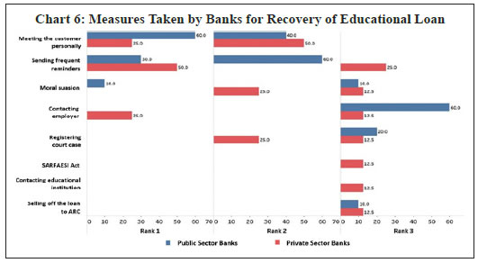
Lenders’ Perspective of Education Loan NPA: Results from a Survey of Banks in Tamil Nadu While the preceding section estimates the default probability based on borrower characteristics using account level data from three banks, this section attempts to present the broader picture of the issue of NPA in education loan from the perspective of the lending banks in Tamil Nadu. In this context, a questionnaire-based survey of PSBs and PVBs operating in the state was undertaken during July 2020 to identify the major reasons for education loan default and the stakeholders that the banks involve in the recovery process. Based on the responses received from 10 PSBs (including one RRB) and 8 PVBs,16 we outline some important observations in this section. The proportion of education loan in total loan portfolio in the respondent banks varies from less than one per cent to 18 per cent and the NPA ratio in education loan segment varies from less than one per cent to 33 per cent at all-India level. Both PSBs and PVBs reported sharp fall in education loan applications since the onset of the COVID pandemic, with PSBs reporting a sharper decline than their counterparts in the private sector. Responding to the question on factors investigated before sanction of education loan, the banks stated that know your customer (KYC) document of the borrower/ guarantor, CIBIL reports, institution quality or ranking, past academic record of the student, repayment ability of the co-borrower and job prospect of the education course are some of the factors primarily considered. According to one PVB, CIBIL score is checked for all the education loan accounts below ₹4 lakh, for which there is no security requirement. According to a number of banks, assessing the future employment opportunity of the student remains a challenging task for the bank and several market related information available in newspaper or internet is used for the same. Few banks classify institutions into different categories based on courses offered, infrastructure, accreditation, affiliation, rankings, faculty, placement track records, average salary offered, prospective employer list and re-employment capacity. There were considerable differences between PSBs and PVBs in their responses to the queries regarding reasons for default, measures taken for recovery of loans and stakeholders involved in the loan recovery process. While 70 per cent of PSBs cited unemployment as the most important reason for defaults in education loan, 50 per cent of PVBs felt willful default was the primary reason. Unemployment, however, figured as the second most important reason for default among 50 per cent of the respondent PVBs. Non-completion of course by the student borrower was cited as the third important factor for loan default among 37.5 per cent of the PVBs as against 10 per cent among PSBs. Not responding to the bank’s reminders was another concern for both PSBs and PVBs. Other reasons given by PSBs for loan default include partial recovery under the one-time settlement offered by them and migration to another country by the student borrower without prior notice to the bank (Chart 5). With regard to loan recovery, meeting the customer personally and sending reminders were two main steps taken by the banks, although the relative importance of these measures differed between PSBs and PVBs. While the majority of PSBs (60 per cent) stated that they relied more on personal meetings with the borrowers as the primary mode of loan recovery, half the PVBs stated that they primarily relied on sending frequent reminders. An equal percentage of these banks also stated that personal meetings with the borrower was the second most important mode of loan recovery. Contacting the employer of the student borrower was the primary mode of loan recovery for one fourth of the PVBs and the third most important mode for loan recovery for 60 per cent of PSBs. A higher percentage of PVBs resort to selling off the loan to asset reconstruction companies (ARCs) than PSBs. Contacting educational institution and imposing the SARFAESI Act are other modes employed by PVBs to recover their loans (Chart 6). 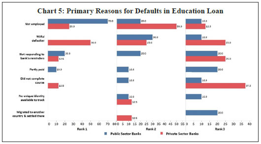
 Responses to a query about the stakeholders that banks have involved in their educational loan recovery process indicate that court’s intervention was sought by 64 per cent of PVBs as against only 29 per cent of PSBs. PSBs appear to rely more on recovery agents (35 per cent) than PVBs (9 per cent). Involvement of asset reconstruction company (ARC) was more in the case of PVBs (18 per cent) than for PSBs (12 per cent) (Chart 7). Section VII
Concluding Observations The study throws light on some aspects of education loan in India, with special reference to Tamil Nadu. Over the years, financing of higher education in India has moved from a primarily government aided model to a privately funded one in which the importance of education loan has increased. However, monitoring such loan accounts remains challenging for bankers due to difficulty in assessing the job market for entrants and rapid migration of student loanees in search of job. Despite the rising NPAs in education loan segment, limited available data hampers a detailed analysis of borrower cohort which is more prone to default. The present study tries to fill this gap by using detailed account level information of education loans of select banks in Tamil Nadu. The major findings of the empirical research presented in the paper have some important policy perspectives. We find that several spatial, borrower and scheme-specific factors are significant predictors of default in the education loan segment. For the two PSBs in our sample, both of which have a significant presence of rural accounts in their education loan portfolio, empirical results suggest rural accounts have a lower probability of default as compared to metropolitan accounts. However, we find it to be the opposite for the PVB in our sample. Further, accounts with higher income of co-borrowers, those backed by collaterals and subsidised accounts are less prone to default. Longer duration reduces default probability while higher interest rate increases the same. Lender’s perspective as elicited from the questionnaire-based survey indicates that default primarily stems from the borrower’s inability to pay (unemployment) as well as unwillingness to do so (willful default). Public sector banks prefer persuasive measures through personal meetings, failing which they adopt more coercive means to recover their loans, particularly in cases of willful defaults. Survey responses indicate private sector banks take legal recourse more often than their public sector counterparts. The results highlight the strategic importance of obtaining borrowers’ Aadhar information for tracking the loan performance and reducing the default risk. The results also show that a more flexible payment schedule with longer moratorium could potentially reduce default. Though the concept of income contingent loans in financing higher education has gained popularity in other countries, the same is yet to take off in India. In the light of our empirical findings, the policy suggestion is to explore the option of introducing such income contingent schemes in India. However, success of such a scheme largely depends on its structure, as country experiences show that ICL generates adverse selection issues in education loan market. The study has some limitations stemming from non-availability of appropriate employment and/or income data. Though the study attempts to identify determinants of default from account level information, the aspect of repayment capacity based on availability of employment opportunities as well as salaries offered remain outside the scope of the present paper. In addition, it is important to gain insights from students who obtain loan for higher studies and are about to enter the job market few years down the line to understand what causes default as well as to design a proper income contingent loan scheme. Future work on these topics could provide more macro and micro evidences on the issues and challenges associated with education loan default in India.
References: Akerlof, George A. (1970). The Market for “Lemons”: Quality Uncertainty and the Market Mechanism. The Quarterly Journal of Economics, Volume 84, Issue 3, August, Pages 488–500, https://doi.org/10.2307/1879431 Amemiya, T. (1981). Qualitative Response Models: A Survey. Journal of Economic Literature, 19(4), 1483-1536. Retrieved on December 16, 2020, from http://www.jstor.org/stable/2724565. Andruska, E. A., Hogarth, J. M., Fletcher, C. N., Forbes, G. R., & Wohlgemuth, D. R. (2014). Do you know what you owe? Students’ understanding of their student loans. Journal of Student Financial Aid, 44(2), 3. Avery, C., & Turner, S. (2012). Student Loans: Do College Students Borrow Too Much--Or Not Enough?. Journal of Economic Perspectives, 26(1), 165- 92. doi: 10.1257/jep.26.1.165 Ballkoci, V., & Gremi, E. (2016). Logit Analysis for Predicting the Bankruptcy of Albanian Retail Firms. Academic Journal of Interdisciplinary Studies, 5(3 S1), 137-137. doi:10.36941/ajis Bandyopadhyay, A. (2016). Studying borrower level risk characteristics of education loan in India. IIMB Management Review, 28(3), 126-135. https://doi.org/10.1016/j.iimb.2016.06.001 Barr, N. (2004). Higher education funding. Oxford review of economic policy, 20(2), 264-283. https://doi.org/10.1093/oxrep/grh015 Ben, Miller (2018). The Student Debt Problem is Worse than We Imagined. New York Times, August 25. Birdsall, N. (1996). Public spending on higher education in developing countries: Too much or Too Little?. Economics of Education Review, 15(4), 407-419. https://doi.org/10.1016/S0272-7757(96)00028-3 Brant, R. (1990). Assessing Proportionality in the Proportional Odds Model for Ordinal Logistic Regression. Biometrics, 46(4), 1171-1178. doi:10.2307/2532457. Box, G. E., & Tidwell, P. W. (1962). Transformation of the independent variables. Technometrics, 4(4), 531-550. doi:10.1080/00401706.1962.10490 038 Cabrera, A. F. (1994). Logistic regression analysis in higher education: A applied perspective. In John C. Smart (ed.), Higher Education: Handbook for the Study of Higher Education. Vol. 10, pp. 225–256. New York: Agathon Press. Chandrasekhar, S., Rani, P. G., & Sahoo, S. (2016). Household expenditure on higher education in India: What do we know & What do recent data have to say. Working Paper-2016-030. Indira Gandhi Institute of Development Research. Retrieved on December 16, 2020 from http://www.igidr.ac.in/pdf/publication/WP-2016-030.pdf. Chapman, B., & Lounkaew, K. (2015). An analysis of Stafford loan repayment burdens. Economics of Education Review, 45, 89-102. https://doi.org/10.1016/j.econedurev.2014.11.003. Clogg, C. C., & Shihadeh, E. S. (1994). Statistical Models for Ordered Variables. Thousand Oaks, CA, Sage Publications. Dyl, E. A., & McGann, A. F. (1977). Discriminant Analysis of Student Loan Applications. Journal of student financial aid, 7(3), 35-40. Dynarski, M. (1994). Who defaults on student loans? Findings from the national postsecondary student aid study. Economics of education review, 13(1), 55-68. https://doi.org/10.1016/0272-7757(94)90023-X. Fahrmeir, L. & G. Tutz, 1994. Multivariate Statistical Modeling Based on Generalized Linear Models, Berlin, Springer Verlag. Field, E. (2009). Educational debt burden and career choice: Evidence from a financial aid experiment at NYU Law School. American Economic Journal: Applied Economics, 1(1), 1-21. DOI: 10.1257/app.1.1.1 Flint, T. A. (1994). The Federal Student Loan Default Cohort: A Case Study. Journal of Student Financial Aid, 24(1), 13-30. Forbes (2019). Student Loan Debt Still Impacting Millennial Homebuyers. March 31. Gouvêa, M. A., & Gonçalves, E. B. (2007). Credit risk analysis applying logistic regression, neural networks and genetic algorithms models. In Production and Operations Management Society, 18th Annual Conference , May. Greene, W. H., & Hensher, D. A. (2010). Modeling ordered choices: A primer. Cambridge University Press. Herr, E., & Burt, L. (2005). Predicting Student Loan Default for the University of Texas at Austin. Journal of Student Financial Aid, 35(2), 27-49. Hillman, N. W. (2014). College on credit: A multilevel analysis of student loan default. The Review of Higher Education, 37(2), 169-195. doi: 10.1353/ rhe.2014.0011 Hillman, N. W. (2015a). Borrowing and Repaying Federal Student Loans. Journal of Student Financial Aid, 45(3), 35-48. Hillman, N. W. (2015b). Cohort default rates: Predicting the probability of federal sanctions. Educational Policy, 29(4), 559-582. https://doi.org/10.1177/0895904813510772 Hosmer, D. W., & Lemeshow, S. (1980). Goodness of fit tests for the multiple logistic regression model. Communications in statistics-Theory and Methods, 9(10), 1043-1069. doi: 10.1080/03610928008827941 Hosmer Jr, D. W., Lemeshow, S., & Sturdivant, R. X. (2013). Applied logistic regression (Vol. 398). John Wiley & Sons. Ionescu, F., & Simpson, N. (2016). Default risk and private student loans: Implications for higher education policies. Journal of Economic Dynamics and Control, 64, 119-147. https://doi.org/10.1016/j.jedc.2015.12.003. Jayadev, M. (2017). An analysis of educational loans. Economic and Political Weekly, 52(51), 108-117. Johnsen, T., & Melicher, R. W. (1994). Predicting corporate bankruptcy and financial distress: Information value added by multinomial logit models. Journal of Economics and Business, 46(4), 269-286. https://doi.org/10.1016/0148-6195(94)90038-8 Khemais, Z., Nesrine, D., & Mohamed, M. (2016). Credit scoring and default risk prediction: A comparative study between discriminant analysis & logistic regression. International Journal of Economics and Finance, 8(4), 39-53. Knapp, L. G., & Seaks, T. G. (1992). An analysis of the probability of default on federally guranteed student loans. The review of economics and statistics, 404-411. https://doi.org/10.2307/2109484 Long, J. S., & Freese, J. (2006). Regression models for categorical dependent variables using Stata. Stata press. Looney, A., & Yannelis, C. (2015). A crisis in student loans?: How changes in the characteristics of borrowers and in the institutions they attended contributed to rising loan defaults. Brookings Papers on Economic Activity, FALL 2015, 1-68. Retrieved on December 17, 2020, from http://www.jstor.org/stable/43752167 McCullagh, P. (1980). Regression models for ordinal data. Journal of the Royal Statistical Society: Series B (Methodological), 42(2), 109-127. https://doi.org/10.1111/j.2517-6161.1980.tb01109.x| Mezza, A., & Sommer, K. (2016). A Trillion-Dollar Question: What Predicts Student Loan Delinquencies?. Journal of Student Financial Aid, 46(3), 16-54. Monteverde, K. (2000). Managing student loan default risk: Evidence from a privately guaranteed portfolio. Research in higher education, 41(3), 331-352. doi: https://doi.org/10.1023/A:1007090811011 Mor, N. (2019). Students Loans for Medical Education in India. Retrieved on December 16, 2020 from https://www.researchgate.net/profile/Nachiket_Mor/publication/335976325_Students_Loans_for_Medical_Education_in_India/links/5d883804458515cbd1b3a9a6/Students-Loans-for-Medical-Educationin-India.pdf. Myers, G., & Siera, S. (1980). Development and Validation of Discriminant Analysis Models for Student Loan Defaultees and Non-Defaultees. Journal of student financial aid, 10(1), 9-17. Ostrom, E. (2010). Beyond Markets and States: Polycentre Governance of Complex Economic Systems. American Economic Review, 100(3), 641-672. Paul, P., Pennell, M. L., & Lemeshow, S. (2013). Standardizing the power of the Hosmer–Lemeshow goodness of fit test in large data sets. Statistics in medicine, 32(1), 67-80. https://doi.org/10.1002/sim.5525 Piirainen, K. A., Raivio, T., Lähteenmäki-Smith, K., Alkaersig, L., & Li- Ying, J. (2018). The reverse tragedy of the commons: A exploratory account of incentives for under-exploitation in an open innovation environment. Technology Analysis & Strategic Management, 30(3), 268-281. https://doi.org/10.1080/09537325.2017.1308479 Pregibon, D. (1981). Logistic regression diagnostics. The Annals of Statistics, 9(4), 705-724. doi:10.1214/aos/1176345513 Quednau, H. D. (1988). An extended threshold model for analyzing ordered categorical data. Biometrical journal, 30(2), 147-155. https://doi.org/10.1002/bimj.4710300204| Seifert, C. F., & Wordern, L. (2004). Two Studies Assessing the Effectiveness of Early Intervention on the Default Behavior of Student Loan Borrowers. Journal of Student Financial Aid, 34(3), 41-52. Stockham, D. H., & Hesseldenz, J. S. (1979). Predicting national direct student loan defaults: The role of personality data. Research in higher education, 10(3), 195-205. https://doi.org/10.1007/BF00976264 Tilak, J. B. G. (2007). The Kothari Commission and Financing of Education. Economic and Political Weekly, 42(10), 874-882. Retrieved December 16, 2020, from http://www.jstor.org/stable/4419340 Verdes, E., & Rudas, T. (2003). The π* index as a new alternative for assessing goodness of fit of logistic regression. In Foundations of Statistical Inference (pp. 167-177). Physica, Heidelberg. https://doi.org/10.1007/978-3-642-57410-8_15 Volkwein, J. F., & Szelest, B. P. (1995). Individual and campus characteristics associated with student loan default. Research in higher education, 36(1), 41-72. https://doi.org/10.1007/BF02207766 Wegmann, C., Cunningham, A., & Merisotis, J. (2003). Private loans and choice in financing higher education. Washington, DC: Institute for Higher Education Policy. Westgaard, S., & Van der Wijst, N. (2001). Default probabilities in a corporate bank portfolio: A logistic model approach. European journal of operational research, 135(2), 338-349. https://doi.org/10.1016/S0377-2217(01)00045-5 Williams, R. (2006). Generalized ordered logit/partial proportional odds models for ordinal dependent variables. The Stata Journal, 6(1), 58-82. Wilms, W. W., Moore, R. W., & Bolus, R. E. (1987). Whose fault is default? A study of the impact of student characteristics and institutional practices on guaranteed student loan default rates in California. Educational Evaluation and Policy Analysis, 9(1), 41-54. doi:10.3102/01623737009001041. Wilson, C. (1989). Adverse selection. In John Eatwell, Murray Milgate, and Peter Newman, eds., Allocation, Information and Markets. London: Macmillan, 1987, pp. 31-34.
| Appendix Table 1: Top 10 Banks in Tamil Nadu in terms of Share on Education Loan Extended during 2019-20 | | (₹ crore) | | Sl. No. | Bank | Education Loan Sanctioned (Numbers) | Education Loan Sanctioned (Amount) | Market Share in terms of Amount (per cent) | | 1 | State Bank of India | 9,832 | 271.08 | 18.4 | | 2 | Canara Bank | 17,274 | 250.20 | 17.0 | | 3 | Indian Bank | 2,430 | 167.45 | 11.4 | | 4 | Indian Overseas Bank | 3250 | 125.45 | 8.5 | | 5 | Bank of Baroda | 3,135 | 98.08 | 6.7 | | 6 | Punjab National Bank | 3006 | 81.41 | 5.5 | | 7 | AXIS Bank | 877 | 62.04 | 4.2 | | 8 | Bank of India | 1288 | 49.04 | 3.3 | | 9 | Tamil Nadu Mercantile Bank Ltd | 450 | 47.69 | 3.2 | | 10 | Syndicate Bank | 765 | 46.28 | 3.1 | | Source: Agenda papers of SLBC, Tamil Nadu. |
| Appendix Table 2: Education Loan Schemes in Sample | | Scheme Code | Description of Scheme | | Bank A | | A1 | IBA model education loan scheme | | A2 | Education loan for premier institutions | | A3 | Education loan under differential interest rate (DRI)/for reserved categories | | A4 | Education loan for physically challenged | | A5 | Education loan for down payment to counselling authorities | | Bank B | | B1 | Education loan under IBA model scheme without credit guarantee cover | | B2 | Uncollaterallised education loan up to ₹7.50 lakh covered under credit guarantee fund scheme. | | B3 | Education loan for admission into an approved college under management quota. | | B4 | Education loan for vocational education courses | | B5 | Education loan for paying coaching fees to prepare for entrance examination of professional courses | | Bank C | | C1 | Education loan for merit-based admission | | C2 | Education loan for admission under management quota |
| Appendix Table 3: Review of Methodologies | | Sl. No. | Author(s) | Year | Methodology | Main Findings | | 1 | Thomas A Flint | 1994 | Logistic regression analysis of survey data | Students' pre-college characteristics are statistically significant in determining probability of default. Though students' grade point average is statistically significant, enrolment choices, amount borrowed, number of loans and reasons for leaving the college are not statistically significant. | | 2 | Seifert and Wordern | 2004 | Logistic regression | Early intervention to check loan default had significant positive impact, though the impact of such intervention on future behaviour of the borrower was found to be relatively small. | | 3 | Emily A. Andruska, Jeanne M. Hogarth, Cynthia Needles Fletcher, Gregory R. Forbes, Darin R. Wohlgemuth | 2014 | Logistic regression and ordered logit regression on survey data | Examining awareness amongst students regarding their student loans, the results of the study suggest that although the majority of students are aware that they owe on student loans, many underestimate the amount they owe. The study examines the roles that counsellors, educators, and policy makers can play in improving students’ understanding of their student loan debt. | | 4 | Nicholas W. Hillman | 2015 | Logistic regression on survey data | Using Integrated Postsecondary Education Data System (IPEDS) data from 2008 (N = 4,488) in the context of US, and applying logistic regression, this study finds for- profit colleges, those accredited by vocational education programmes, and those serving diverse student bodies experience more student loan default. | | 5 | Mezza and Somer | 2016 | Multivariate Tobit model | Credit scores of young borrowers are an important determinant of future student loan delinquency. | | 6 | Arindam Bandyopadhay | 2016 | Multivariate logit and tobit regression on bank lending data | Education loan defaults are mainly influenced by security, borrower margin, and repayment periods. The presence of guarantor or co-borrower and collateral significantly reduce default loss rates. The socioeconomic characteristics of borrowers and their regional locations also act as important factors associated with education loan defaults. The results suggest that by segmenting borrowers by probability of default and loss given default in a multi-dimensional scale, banks can adopt better risk mitigation and pricing strategies to resolve borrower problems. | | 7 | Looney and Yannelis | 2015 | Logistic regression analysis | Types of institution, debt level and labour market conditions explain a large share of the rise in student loan default in U.SA. |
| Appendix Table 4: Default Rate in Selected Banks | | (Per cent) | | Sl. No. | Proportion of NPA | Bank A | Bank B | Bank C | | 1 | Overall | 20.94 | 9.6 | 43.62 | | 2 | Subsidy eligible loans | 18.62 | 9.22 | 52.63 | | 3 | Non-subsidised loans | 27.05 | 10.78 | 37.65 | | 4 | Rural | 21.37 | 9.27 | 60.68 | | 5 | Semi-urban | 20.38 | 9.4 | 39.33 | | 6 | Urban | 21.97 | 8.57 | 43.23 | | 7 | Metropolitan | 20.93 | 19.61 | 25.62 | | 8 | Male | 20.65 | 9.98 | 46.91 | | 9 | Female | 20.66 | 8.88 | 37.13 | | 10 | Above median income | 14.42 | 9.07 | 20.10 | | 11 | Below median income | 25.2 | 10.07 | 55.67 |
| Appendix Table 5: Box-Tidwell Regression Results for Bank C | | Continuous Variables | Nonlinear Deviation | P value | P1 | | ln_inc | 75.099 | 0.000 | 4.660 | | ln_int | 5.784 | 0.016 | 4.239 | | in_dur | 0.125 | 0.724 | 1.286 |
| Appendix Table 6: Collinearity Diagnostics | | | Bank A | Bank B | Bank C | | VIF | Tolerance | VIF | Tolerance | VIF | Tolerance | | Ln_dur | 1.010 | 0.992 | 1.000 | 0.998 | 1.070 | 0.933 | | Ln_inc | 1.020 | 0.990 | 1.000 | 0.999 | 1.100 | 0.910 | | Ln_int | 1.020 | 0.983 | 1.000 | 0.999 | 1.030 | 0.971 | | Mean VIF | 1.010 | 1.000 | 1.070 |
* The authors are Assistant Adviser and Director, respectively in the Department of Economic and Policy Research (DEPR), Reserve Bank of India (RBI), Chennai. Assistance in data compilation extended by Shri B. Sathish, Assistant, DEPR, RBI, Chennai, inputs provided by Shri. S. Subbiah, Manager, RBI, Chennai and support provided by Shri K. Sriram, Smt. Sharmila Prasad and Shri C. Rajkumar, DEPR, RBI, Chennai in conducting the survey are gratefully acknowledged. The authors are also thankful to the Department of Supervision (Banking), RBI, Chennai, for help in obtaining the data from banks. The authors also benefitted from the valuable suggestions received from Dr. M. K. Saggar, Executive Director, RBI, Shri SMN Swamy, Regional Director, RBI, Chennai, internal discussant Shri Rishabh Kumar, Manager, DEPR, RBI and external anonymous referee. The views expressed in this paper are their own and do not reflect those of the organisation they belong to. 1 2020 Human Development Data: http://hdr.undp.org/en/data. 2 As proportion to the corresponding population age. 3 As at end-March 2020, Tamil-Nadu accounted for almost 19 per cent of total education loans extended by scheduled commercial banks in India, which is the highest among states. Latest available data shows that its share in total NPAs in the education loan segment stood at 50 per cent as at end-September 2017, which provides the context and justification for this study. 4 Education loans availed from October 2019 onwards are linked to external benchmark. 5 Source: Basic Statistical Return of Scheduled Commercial Banks in India. 6 Source: Agenda papers, State Level Bankers’ Committee (SLBC), Tamil Nadu. Available at www.slbctn.com. 7 Source: Same as footnote 6. 8 Moratorium period refers to course period plus one year. 9 Source:5th Annual Report (2018-19) of National Credit Guarantee Trust Company Limited (NCGTCL) 10 Source: Student Loan Debt Statistics 2020 available at https://educationdata.org/studentloan-debt-statistics/ 11 A Stafford Loan is a student loan offered to eligible students enrolled in accredited American institutions of higher education to help finance their education. 12 Table 3 provides key NPA statistics (in terms of amount outstanding) while Appendix Table 4 provides default rates (in terms of frequency). 13 Amemiya (1981) shows that by multiplying the logit estimates by 0.625, one may obtain the corresponding probit estimations. 14 The Hosmer Lemeshow (HL) test statistic (Hosmer and Lemeshow 1980; Hosmer et al., 2013), which is widely used in risk modelling to test the predictive power of the model by comparing the observed and expected probabilities, is significant for the model used for Bank A and Bank B, while insignificant for the model used for Bank C. This indicates somewhat poor fit for the model used for Bank A and Bank B. However, since in the present case, the logistic models are not used for prediction purpose, results are reported following a significant value of LR chi2. Further, it is often found that HL statistic is not neutral to the choice of bins which is somewhat arbitrary and has low power (Verdes and Rudas 2003, Paul et al., 2013). 15 Use of male dummy does not alter the results, as all coefficients of male dummy are found to be statistically insignificant, with p values of 0.296, 0.545 and 0.882, respectively for the three Panels. 16 The questionnaire was sent to all member banks of the State Level Bankers’ Committee, of which responses were obtained from 18 public sector and private sector banks which accounted for nearly 78 per cent of the outstanding education loans in Tamil Nadu as on March 2020. |