Saurabh Sharma and Ipsita Padhi* Received on: September 17, 2020
Accepted on: December 8, 2020 Assessing macroeconomic demand conditions is critical for monetary policy to gauge imminent inflationary pressures. Generally, measures of output gap, calculated by applying statistical filters on GDP data, are used for this purpose. GDP data, however, are released only at quarterly frequency with a lag of approximately two months. This paper proposes an alternative indicator of economic slack that captures demand conditions efficiently and is also available at higher frequency. A macroeconomic demand index constructed for this purpose using a rich set of high frequency (monthly) indicators emerges as a better predictor of core inflation than other measures. JEL Classification: C32, C53, E31, E32, E37 Keywords: Demand index, Phillips curve, factor model, inflation forecast Introduction Traditionally, output gap and capacity utilisation are widely used to assess economic slack. Output gap is generally calculated by applying statistical filters (Hodrick-Prescott, Band-Pass, Multivariate Kalman Filter, etc.) on GDP data, while capacity utilization is derived mainly from surveys on corporate performance. One of the biggest limitations of these measures, however, is that they are available with a time lag. The national accounts data for any quarter is released with a lag of approximately two months after the end of the reference quarter. Similarly, data on capacity utilization from the Order Books, Inventories and Capacity Utilisation Survey (OBICUS) of RBI is released with a lag of more than one quarter. In view of the importance of inflation forecasts to the conduct of monetary policy under a flexible inflation targeting (FIT) framework, and the well-established role of economic slack in influencing the near-term evolution of the inflation trajectory, it is useful to explore alternative measures which not only capture economic slack efficiently, but also can be available at higher frequency. This paper attempts to create a macroeconomic demand index using a set of high frequency indicators (HFIs), which are available at monthly frequency. We use an unobserved components model that combines a Bayesian dynamic factor model (DFM) with a Phillips curve equation to estimate the measure of economic slack. While the Bayesian dynamic factor model extracts a common factor from various high frequency indicators, the Phillips curve equation ensures that this common factor contains information about inflation dynamics. The idea is to estimate not just any measure of economic slack but one that closely resembles inflationary pressures. In the second part of the paper, we test the predictive ability of the estimated demand index by assessing the inflation-forecasting performance of the constructed demand index vis-à-vis other measures of excess demand like HP filtered output gap and capacity utilization. The forecasting performance assessment exercise clearly establishes the superior predictive power of the constructed measure of economic slack relative to conventional measures of demand. The organisation of the remaining part of the paper is as follows. Section II surveys the relevant literature. Section III describes the econometric model used in the paper. Section IV explains the methodology. Section V presents the empirical results and section VI concludes. Section II
Literature Survey The multivariate unobserved components model used in this paper is a synthesis of two different strands of literature – DFMs and Phillips curve. DFMs have been used widely to construct indices of economic activity and more recently to nowcast GDP (Stock and Watson, 1989; Giannone, Reichlin and Small, 2008 in the international context and Biswas, Banerjee and Das, 2012; Bhadury, Ghosh and Kumar, 2020 in the Indian context). Our paper is related to this strand of literature but with one important distinction. We are concerned not only with obtaining the estimate of real activity, but also whether that estimate contains important information about inflationary pressures. In order to incorporate this into the model, we introduce the Phillips curve equation (relating inflation and output gap) into the Bayesian DFM state-space framework. Several studies have used a bivariate framework to extract output gap by using a Phillips curve equation along with the equation relating actual and potential output. Kuttner (1994) initiated this literature by using a bivariate unobserved components model to estimate potential output. Planas (2008) estimated a Bayesian version of Kuttner’s model. Building upon this framework, Jarocinski and Lenza (2015) used a DFM equation in the bivariate model to extract the output gap from multiple indicators of economic activity and forecasted core inflation using it. We follow a similar approach. In doing so, we borrow from the extensive literature on Phillips curve, both in India and abroad. In the Indian context, several studies have found support for the Phillips curve hypothesis (Patra and Kapur, 2012 using WPI data and Behera, Wahi and Kapur, 2017 using CPI data). The specification of the Phillips curve equation in our model draws from these studies, but is estimated using a state-space framework. Section III
The Econometric Model We construct a macroeconomic demand index that contains useful information about inflationary pressures. We use the following multivariate unobserved components model to extract the measure of economic slack. Section IV
Estimation Strategy After specifying the broad modelling framework in the previous section, we turn to the detailed methodology in this section. The first sub-section explains the identification strategy; sub-section 2 describes the exact specification of the Phillips curve equation; sub-section 3 relates to the selection of HFIs; sub-section 4 presents the final specification and estimation technique of the model, and the last sub-section describes the data. IV.1 The identification strategy The broad identification strategy for our empirical estimation rests on the following premise. First, various types of high frequency indicators possess some common information about the macroeconomic demand conditions. Second, core inflation in India reacts well to changing demand conditions, which means there exists a robust Phillips curve type relationship between them. The first assertion is validated by the way in which we select our high frequency indicators. The second presumption gains credibility from the vast Indian literature which suggests that there exists a robust Phillips curve relationship in India both for core and headline inflation (Kapur and Patra, 2010; Behera, Wahi and Kapur, 2017; Pattanaik, Muduli and Ray, 2019). Taking a cue from these studies, we also estimate the Phillips curve for core inflation using a state-space framework. This not only reinforces the literature but also guides us about the exact specification to be used later for estimation of demand index. IV.2 The Phillips Curve We begin with the classic “triangle” model of inflation (Gordon, 1997), which relates inflation to three basic determinants: inertia, excess demand and supply shocks. 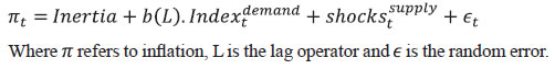 In using this framework for our purpose, we face four major modelling choices: (i) Which measure of inflation should be used, headline or core?; (ii) What is the measure of excess demand to be used?; (iii) What are the supply shocks, if any, to be included?; and (iv) How to capture the inertia component? To resolve these queries, we take guidance from the literature. Where the literature does not provide a clear-cut answer, we decide based on the forecasting performance (for inflation) of alternate measures/specifications. Given that we are primarily concerned about the ability of the demand index in assessing inflationary impulses, inflation forecasting ability seems to be an appropriate test to determine the reliability of the model. Thus, forecasting performance is used as the metric of evaluation to decide upon the correct specification. We use inflation excluding food and fuel (also referred to as core inflation) as our measure of inflation. Core inflation is expected to be more responsive to demand conditions as it is relatively immune to supply side shocks emanating from food and fuel sectors. This has been corroborated by various studies which find that the impact of excess demand is higher on core inflation compared to headline inflation (Kapur, 2012; Behera et al., 2017). We, therefore, use core inflation to extract information about excess demand/ economic slack in the economy. For the measure of excess demand, both output gap and unemployment gap have been used in the literature. Okun’s Law holds that the output gap and unemployment gap are closely related. Accordingly, we use HP filtered output gap (applied on real GDP) as a proxy for demand. According to Gordon (1997), inflation depends not only on the level but also on the change in excess demand, and models that do not include the change variable are misspecified. In order to account for the rate-of-change effect, we include both contemporaneous and lagged value of output gap in our specification. We now turn to the inclusion of supply shocks. We use core inflation as our measure of inflation which largely excludes supply-side inflationary pressures like food and fuel. However, CPI excluding food and fuel includes petrol and gold whose movements are largely determined by supply factors. Some other supply controls that are widely used in the literature include exchange rate and crude-oil inflation. Food inflation has also been included as a control variable in a few studies to assess potential spillovers to core inflation (Behera et al., 2017). In order to choose the exact specification of our Phillips curve equation, we use the state-space framework with alternative combinations of all these control variables (change in exchange rate, gold, petrol, food and crude oil prices). We compare the forecasting performance of these specifications and conclude that a specification with only exchange rate is the best specification as it has superior forecasting performance (Table 1). Turning next to the inertia component, we observe that it has been modelled in various ways in the literature. While Gordon (1997) simply used the lagged values of inflation to capture the inertia, hybrid versions of the New Keynesian Phillips Curve (NKPC) have used a combination of forward and backward looking variables (Gali and Gertler, 1999). In the Indian context, Patra et al. (2014) used lagged inflation along with one-period lead inflation in the estimation of the NKPC equation, Behera et al. (2017) used only the lagged inflation term to estimate the Phillips curve equation, and Pattanaik et al. (2019) used survey-based household inflation expectations in the Phillips curve specification. In our model, we define inertia in three alternate ways and then check for their forecasting performance in order to select the best specification. In the first case, we use lagged inflation as the measure of inertia in the tradition of Gordon (1997). In the second case, we follow the approach of Jarocinski and Lenza (2015) to model inertia using trend inflation. The trend inflation is assumed to be a random walk process without drift, specified as follows: 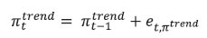
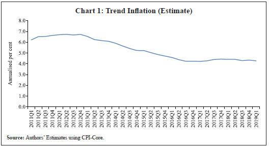
| Table 1: Relative RMSE of alternate specifications | | Model Specification | Relative RMSE | | No supply shocks + inertia (trend inflation) | 1 | | No supply shocks + inertia (inflation expectations) | 1.29 | | No supply shocks + inertia (lagged inflation) | 2.13 | | Supply shocks (petroleum inflation, gold inflation, food inflation, change in rupee-dollar exchange rate) + inertia (trend inflation) | 0.92 | | Supply shocks (petroleum inflation, gold inflation, lagged food inflation, lagged change in rupee-dollar exchange rate) + inertia (trend inflation) | 1.07 | | Supply shocks (petroleum inflation, change in rupee-dollar exchange rate) + inertia (trend inflation) | 0.91 | | Supply shocks (petroleum inflation) + inertia (trend inflation) | 1.03 | | Supply shocks (change in rupee-dollar exchange rate) + inertia (trend inflation) | 0.87 | | Supply shocks (Indian basket crude oil inflation, change in rupee-dollar exchange rate) + inertia (trend inflation) | 0.88 | | Supply shocks (Indian basket crude oil inflation) + inertia (trend inflation) | 1.04 | | Source: Authors’ Estimates. | A number of studies have modelled trend inflation as a random walk process (Cogley et al., 2010; Stock and Watson, 2007). Defining it in this way removes restriction imposed by mean-reversion associated with stationary specification. Since trend inflation is a medium-term concept that is relatively unaffected by short-term dynamics, a random walk process results in a smoother estimate (Chart 1). Another way of modelling trend inflation is to relate it to long-run inflation expectations (Faust and Wright, 2013; Clark and Doh 2014; Jarocinski and Lenza, 2015). We follow this approach in the third case, wherein trend inflation is again used as the measure of inertia, but this time it is modelled using household inflation expectations. Accordingly, we use the following equation to derive trend inflation: 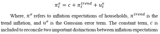 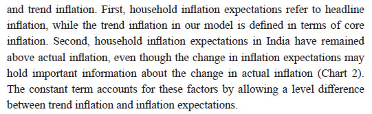
 In addition to these alternate measures of intrinsic persistence, lags of demand index/output gap are also used to account for extrinsic persistence. We then estimate the Phillips curve equation and forecast core inflation using these alternate specifications. The specification with trend inflation modelled as a random walk process has the best root mean squared error (RMSE) score among the competing specifications (Table 1). Trend inflation that incorporates inflation expectations does not improve upon the forecasting performance. This is in line with Pattanaik et al. (2019) who find that ‘the overall explanatory powers of NKPC models with household inflation expectations do not improve relative to similar models with backward looking inflation expectations’. We therefore, specify inertia in our model as trend inflation which is a random walk process without drift. IV.3 Selection of High-frequency Indicators Having finalised the specification of the Phillips curve, we turn to the selection of high frequency indicators. There exist a variety of high-frequency indicators covering different aspects of the economy. The choice of HFIs, therefore, becomes important in order to have a parsimonious specification without losing out on information content. In order to select the HFIs, we broadly follow two steps. First, we peruse the literature to short-list the indicators that could potentially hold relevant information about demand conditions. Second, since we are primarily concerned with obtaining a demand index that can predict core inflation reasonably well, we check the correlation of these indicators with core inflation and HP filtered output gap (henceforth, HP-gap). We select those HFIs which are found to be significantly correlated with core inflation or the output gap. The literature on coincident economic indicators makes use of a variety of high-frequency indicators (see Bhadury et al., 2020 for a detailed survey). We categorise the high-frequency indicators generally used in the literature into the major components of demand: consumption, investment, government spending, and trade.1 HFIs that cannot be binned into these categories but may be potentially useful to capture demand conditions are listed in the miscellaneous category (Table 2). | Table 2: Classification of HFIs under major heads of aggregate demand | | Consumption | Investment-based | Government Spending | Trade | Miscellaneous | • IIP consumer goods
o Durables
o Non-durables
• Petroleum consumption
• Passenger vehicle sales
• Two-wheeler sales
• Government tax revenue
• Air passenger traffic (domestic) | • IIP general
• IIP intermediate goods
• IIP capital goods
• IIP basic goods
• Commercial vehicle sales
• Crude steel production
• Cement production
• Farm tractor sales | • Government total expenditure
• Government revenue expenditure | • Non-oil imports
• Non-oil exports | • Non-food bank credit
• M3 (broad money)
• 91 T-bill yield
• Railway freight | Since the emphasis is to estimate a measure of economic slack, we work with the cyclical dynamics present in each HFI, extracted using HP-filter. As a first round of screening, we check the contemporaneous correlation of respective HFIs with HP-gap (Table 3). Out of these 23 HFIs, six HFIs (freight traffic, SCB non-food credit, M3, 91 T-bill yield, IIP intermediate, and non-oil exports) are contemporaneously negatively correlated with the HP-gap. In order to check the possibility that these HFIs may be associated positively with lead/lag of HP-gap, we calculate the respective cross-correlations. We find that these HFIs are either uncorrelated or negatively correlated with HP-gap at all appropriate lead-lag (Table A.1). From this, we conclude that these HFIs do not possess relevant information about the excess demand in the economy and rather show idiosyncratic dynamics for our period of study. For the remaining 17 HFIs, we also compute correlation with core inflation to assess if they possess information about inflation pressures (Table A.2). We finally obtain a list of 12 HFIs comprising of two-wheeler sales, domestic passenger vehicle sales, domestic commercial vehicles sales, tractor sales, petrol consumption, crude-steel production, air-passenger traffic, IIP-basic, IIP-capital, IIP-consumer durables, IIP- consumer non-durables, IIP-general, that are found to be significantly correlated with either output gap or core inflation. These 12 HFIs are used to compute our first measure of economic demand, which we name DI-12. | Table 3: Correlation of HFIs with HP-filter output gap | | HFI | Correlation with HP-gap | HFI | Correlation with HP-gap | | Domestic Two Wheelers Sales | 0.45*** | SCB Non Food Credit | -0.56*** | | Domestic Passenger Vehicle Sales | 0.63*** | M3 | -0.34** | | Domestic Commercial Vehicle Sales | 0.46*** | 91 T-bill avg. yield | -0.31** | | Farm Tractor Sales | 0.11 | IIP Basic | 0.60*** | | Freight Traffic | -0.30** | IIP Capital | 0.52*** | | Petroleum Consumption | 0.63*** | IIP Intermediate | -0.25 | | Crude Steel Production | 0.38* | IIP Consumer durables | 0.51*** | | Cement Production | 0.02 | IIP Consumer non-durables | 0.23 | | Passenger Traffic Domestic | 0.74*** | IIP General | 0.55*** | | Government Tax Revenue | 0.09 | Government Total Expenditure | 0.06 | | Government Revenue Expenditure | 0.04 | Non-oil Exports | -0.05 | | Non-oil imports | 0.15 | | | Note:*: p < 0.10, **: p < 0.05, ***: p <0.01.
Source: Authors’ Estimates. | Of these 12 HFIs, 4 HFIs (sales associated with two wheelers, passenger vehicles, commercial vehicles and farm tractors) pertain to the automobile industry. On the one hand, this may be beneficial for our case, as these kinds of sales form a good indicator of the private macroeconomic demand. On the other hand, this also opens up the risk of making one-third of the total HFIs prone to fluctuations in one industry. This may prevent our estimate from being representative of the entire economy. We believe that the degree of this trade-off will depend on whether these four HFIs are well correlated among themselves or not. In case they are highly correlated among themselves, the estimation of latent factor may become more biased towards dynamics common to the automobile sector. We find that HFIs pertaining to the automobile sector are well correlated among themselves (Table 4). Two-wheeler sales share the highest correlation on an average with other sectoral HFIs. Moreover, commercial vehicle sales and passenger vehicle sales not only share a high correlation among each other, but also show nearly same level of average correlation with their sectoral counterparts. This suggests that the two HFIs possess almost similar kind of dynamics and removing one of them will not lead to a substantial loss of information. In order to reduce the possible bias of the latent factor, we consider a case in which we drop passenger vehicle sales and two-wheeler sales from the list of HFIs used for the estimation. Thus, we estimate our model using two sets of HFIs. One set includes all the 12 HFIs (DI-12) while the other set uses 10 HFIs (DI-10) after excluding passenger vehicle sales and two-wheeler sales2. | Table 4: Correlation among HFIs in the automobile sector | | | Two-wheelers | Passenger vehicles | Commercial vehicles | Farm tractors | | Two-wheelers | 1 | | | | | Passenger vehicles | 0.67 | 1 | | | | Commercial vehicles | 0.61 | 0.72 | 1 | | | Farm tractors | 0.63 | 0.37 | 0.38 | 1 | | Average Correlation with other Automobile Industry HFIs | 0.64 | 0.59 | 0.57 | 0.46 | | Source: Authors’ Estimates. | IV.4 Final Specification and Estimation Based on the above analysis, we obtain the final specification of the state space model as follows: The Markov chain samples sequentially from the conditional distributions for (parameters/factors) and (factors/parameters) and, at each stage, uses the previous iterations drawing as the conditioning variable, ultimately yields drawings from the joint distribution for (parameters, factors). Thus, the joint distribution conditioned on the p first observations can be approximated by, For the estimation, we choose loose priors so that the estimated parameters are determined more by the data, rather than by the choice of the priors (Table 5). IV.5 Data The data used in the paper pertains to 23 HFIs listed in Table 3, and also output gap, core inflation, food inflation, change in exchange rate, crude oil inflation, gold inflation and petroleum inflation for the period 2011:Q1 to 2019:Q4. The data description and sources are presented in appendix Table A.3. While the HFIs and price indices used in the paper are available at monthly frequency, most of the empirical analysis is carried out using data aggregated to quarterly frequency. This is done to ensure comparability of the estimated results with other conventional measures of slack, which are available only at quarterly frequency. The data transformation associated with HFIs includes aggregating them to quarterly frequency, taking log, de-seasonalizing using X-13 ARIMA and finally applying HP-filter to extract cyclical dynamics. The inflation figures are calculated by aggregating monthly price indices to quarterly frequency, taking log, de-seasonalising them using X-13 ARIMA, and then taking the first difference. This yields the quarter-on-quarter inflation figures. | Table 5: Parameter Estimates | | | Parameter | Prior Distribution | Prior Mean | Prior SD | Posterior Mean
(with 12 indicators) | Posterior Mean
(with 10 indicators) | | Philips curve: |  | Beta | 0.150 | 0.09 | 0.1287 | 0.1308 | | Core Inflation |  | Beta | 0.150 | 0.09 | 0.1101 | 0.1051 | | Gamma | 0.005 | 0.004 | 0.0036 | 0.0035 | | Demand |  | Normal | 0 | 0.9 | 1.1255 | 0.9541 | | Index |  | Normal | 0 | 0.9 | -0.3495 | -0.2463 | | Gamma | 0.005 | 0.004 | 0.0040 | 0.0044 | | Trend Inflation |  | Gamma | 0.005 | 0.004 | 0.0014 | 0.0014 | | Supply Controls |  | Beta | 0.5 | 0.15 | 0.3382 | 0.3395 | | Gamma | 0.02 | 0.01 | 0.0321 | 0.0322 | | Source: Authors’ Estimates. | Section V
Results The posterior estimates of some important parameters3 are presented in Table 5. Results pertaining to different variants of the model (DI-10 and DI-12) suggest that the estimated parameters are robust (in general) to the choice of HFIs used in the model. This adds credibility to our estimation. The normalized factor loadings across the two sets of demand indicators are shown in Chart 3. Factor loadings show the contribution of different economic indicators in the estimated demand index. Broadly, the economic indicators related to IIP constitute the highest share in the demand index followed by crude steel production and automobile sales indicators. The time-varying estimates of the estimated demand indices are plotted in Chart 4.
The estimated demand indices are found to move closely with the conventional measures of economic slack such as HP-gap and capacity utilization from the OBICUS4 (Chart 5).
| Table 6: Correlation between Core Inflation and Different Measures of Economic Slack | | | Demand Index
(12- indicator) | Demand Index
(10- indicator) | HP
Output Gap | OBICUS
Capacity Utilization | Core Inflation | | Demand Index (12-indicator) | 1 | | | | | | Demand Index (10-indicator) | 0.98 | 1 | | | | | HP Output Gap | 0.79 | 0.81 | 1 | | | | OBICUS Capacity Utilisation | 0.76 | 0.77 | 0.59 | 1 | | | Core Inflation | 0.49 | 0.45 | 0.26 | 0.28 | 1 | | Source: Authors’ Estimates. | The estimated demand indices are also found to be well correlated with HP-gap and OBICUS CU (Table 6). In terms of correlation with core inflation, both demand indices are found to be better than both HP-gap and OBICUS CU. Further, regression analysis suggests that the estimated demand indices have greater explanatory power than other conventional measures of demand (Table 7). | Table 7: Regression Estimates | | | (1) | (2) | (3) | (4) | | pi_core | pi_core | pi_core | pi_core | | AR(1) | 0.973***
(0.004) | 0.973***
(0.004) | 0.973***
(0.004) | 0.969***
(0.004) | | MA(1) | -0.963***
(0.017) | -0.962***
(0.016) | -0.999***
(0.000) | -0.957***
(0.019) | | DI-12 | 0.314***
(0.089) | | | | | DI-10 | | 0.362***
(0.102) | | | | HP-gap | | | 0.116*
(0.0635) | | | OBICUS_CU | | | | 0.089***
(0.030) | | Adj. R2 | 0.651 | 0.650 | 0.557 | 0.613 | | N | 35 | 35 | 35 | 35 | Note: Standard errors in parentheses; * p < 0.10, ** p < 0.05, *** p < 0.01;
ARIMA specification has been chosen based on SIC criterion.
Source: Authors’ Estimates. | V.1 Forecasting Exercise In this section, we evaluate various measures of economic slack in terms of their performance in forecasting core inflation, following Coenen, Smets, and Vetlov (2009). As a first step, we determine the ARIMA specification that best describes the data generating process of core inflation. We use this ARIMA specification for generating 1 to 4 quarters-ahead rolling forecasts. Subsequently, we nest this ARIMA specification with different measures of economic slack to form different bivariate models (of core inflation and economic slack measures). The forecasting performance of these different bivariate models are then evaluated and compared to know whether inclusion of economic slack helps predict core inflation better or not. If it does, then which measure of economic slack does it the best? These are some of the questions which have direct practical utility for the central bank. The general specification of the bivariate model is as follows, Total number of rolling samples are 13 while total length of our data is 36 quarters (2011Q1-2019Q4). This means we practically use 36 per cent of our data in conducting and evaluating out-of-sample forecasts. Moreover, the period 2015:Q4 to 2018:Q4 includes both upturns and downturns in economic slack (Chart 6). This ensures that forecasting evaluation/performance is independent of the state of the economic slack, and lends robustness and credibility to our forecasting results. The indicative charts for rolling forecast evaluation are presented below (Chart 7). RMSE results are presented in Table 8. The results suggest that inclusion of economic slack generates mixed results as far as forecasting core inflation is concerned. While model with OBISCUS CU performs badly than univariate ARIMA, model with HP-gap performs better than ARIMA at two, three and four quarter-ahead horizons. However, the estimated demand indices (DI-10, DI-12) perform better than ARIMA and model with HP-gap at all forecasting horizons. Moreover, among the two, DI-10 performs better, making it the best forecaster of core inflation given the framework and time-period considered in our study.
| Table 8: RMSE of Forecasts | | Specification | Forecast Horizon | | Q1 | Q2 | Q3 | Q4 | | ARIMA | 0.352 | 0.387 | 0.416 | 0.463 | | HP Output gap | 0.359 | 0.372 | 0.412 | 0.410 | | OBICUS capacity utilisation | 0.413 | 0.461 | 0.504 | 0.499 | | Demand Index (12-indicators) | 0.348 | 0.355 | 0.396 | 0.391 | | Demand Index (10-indicators) | 0.320 | 0.333 | 0.362 | 0.370 | | Source: Authors’ Estimates. | Section VI
Conclusion Assessing macroeconomic demand conditions is critical for monetary policy to gauge imminent inflationary pressures. Generally, measures of output gap, calculated by applying statistical filters on GDP data, are used for this purpose. However, one of the limitations of these conventional measures of output gap is that the national accounts data used in their calculation are released only at quarterly frequency with a lag of approximately two months. In this paper, we create a macroeconomic demand index using a rich set of high frequency (monthly) indicators by employing a multivariate unobserved components model. In doing so, we face a number of modelling choices regarding different specifications of the structural model, variables used, and assumptions about the underlying structural processes. We resolve these questions based on the forecasting ability of the alternate specifications. We find that the demand index constructed in this paper is a better predictor of core inflation than conventional measures of economic slack like HP-gap and capacity utilization. The constructed measures of demand conditions, not only provide lead information about the state of economic slack in the economy, but also seem to be an important indicator of inflationary pressures.
References Behera, H. K., Wahi, G., & Kapur, M. (2017). Phillips curve relationship in India: Evidence from state-level analysis. RBI Working Paper Series, WPS (DEPR): 08 / 2017. Bhadury, S., Ghosh, S., & Kumar, P. (2020). Nowcasting Indian GDP growth using a Dynamic Factor Model. RBI Working Paper Series No. 03. Biswas, D., Banerjee, N., & Das, A. (2012). Real Time Business Conditions Index: A Statistically Optimal Framework for India. RBI, 38. Coenen, G., F. Smets, & I. Vetlov. 2009. Estimation of the Euro Area Output Gap Using the NAWM. Working Paper No. 5, Bank of Lithuania Gali, J., & Gertler, M. (1999). Inflation dynamics: A structural econometric analysis. Journal of monetary Economics, 44(2), 195-222. Giannone, D., Reichlin, L., & Small, D. (2008). Nowcasting: The real-time informational content of macroeconomic data. Journal of Monetary Economics, 55(4), 665-676. Gordon, R. J. (1997). The time-varying NAIRU and its implications for economic policy. Journal of economic Perspectives, 11(1), 11-32. Jarocinski, M., & Lenza, M. (2015). Output gap and inflation forecasts in a Bayesian dynamic factor model of the euro area. Manuscript, European Central Bank. Kapur, M. (2012). Inflation forecasting: Issues and challenges in India. Reserve Bank of India Working Paper, (01). Kapur, M., & Patra, M. D. (2010). A monetary policy model without money for India (No. 10-183). International Monetary Fund. Kuttner, K. N. (1994). Estimating potential output as a latent variable. Journal of business & economic statistics, 12(3), 361-368. Otrok, C., & Whiteman, C. H. (1998). Bayesian leading indicators: measuring and predicting economic conditions in Iowa. International Economic Review, 997-1014. Patra, M. D., & Kapur, M. (2012). A monetary policy model for India. Macroeconomics and Finance in Emerging Market Economies, 5(1), 18-41. Patra, M. D., Khundrakpam, J. K., & George, A. T. (2014, August). Post-global crisis inflation dynamics in India: What has changed. In India Policy Forum (Vol. 10, No. 1, pp. 117-203). National Council of Applied Economic Research. Pattanaik, S., Muduli, S., & Ray, S. (2019). Inflation Expectations of Households: Do They Influence Wage-Price Dynamics in India? RBI Working Paper Series. Planas, C., Rossi, A., & Fiorentini, G. (2008). Bayesian analysis of the output gap. Journal of Business & Economic Statistics, 26(1), 18-32. Stock, J. H., & Watson, M. W. (1989). New indexes of coincident and leading economic indicators. NBER macroeconomics annual, 4, 351-394. Stock, J. H., & Watson, M. W. (2010). Modelling inflation after the crisis. National Bureau of Economic Research, No. w16488.
Appendix | Table A.1: Correlation with lead/lag of output gap | | HFI | HP-gap(-2) | HP-gap(-1) | HP-gap | HP-gap(+1) | HP-gap(+2) | | Freight Traffic | -0.28 | -0.31 | -0.30 | -0.43 | -0.56 | | | (0.12) | (0.09) | (0.09) | (0.01) | (0.00) | | SCB Non Food Credit | -0.39 | -0.47 | -0.56 | -0.62 | -0.66 | | | (0.03) | (0.01) | (0.00) | (0.00) | (0.00) | | M3 | -0.22 | -0.24 | -0.34 | -0.31 | -0.25 | | | (0.23) | (0.18) | (0.06) | (0.09) | (0.17) | | 91 T-bill avg. yield | -0.02 | -0.20 | -0.31 | -0.35 | -0.56 | | | (0.91) | (0.27) | (0.09) | (0.05) | (0.00) | | IIP Intermediate | -0.57 | -0.35 | -0.25 | -0.36 | -0.29 | | | (0.00) | (0.05) | (0.16) | (0.04) | (0.11) | | Non-oil Exports | 0.07 | 0.10 | -0.05 | -0.24 | -0.25 | | | (0.69) | (0.60) | (0.79) | (0.20) | (0.18) | | Note: Figures in parenthesis are p-values. |
| Table A.2: Correlation with core inflation | | HFI | Correlation with core inflation | HFI | Correlation with core inflation | | IIP Basic | 0.41 | Farm Tractor Sales | 0.32 | | | (0.0185) | | (0.0717) | | IIP Capital | 0.41 | IIP General | 0.46 | | | (0.0212) | | (0.0088) | | Cement Production | 0.14 | Government Total Expenditure | -0.10 | | | (0.4593) | | (0.5758) | | Crude Steel Production | 0.31 | Government Revenue Expenditure | -0.13 | | | (0.0852) | | (0.4906) | | Domestic Commercial Vehicle Sales | 0.48 | Non-oil imports | 0.09 | | | (0.0058) | | (0.6101) | | Domestic Passenger Vehicle Sales | 0.49 | IIP Consumer non-durables | 0.30 | | | (0.0043) | | (0.0927) | | Domestic Two Wheelers Sales | 0.39 | Passenger Traffic Domestic | 0.42 | | | (0.0290) | | (0.0172) | | IIP Consumer durables | 0.27 | Petroleum Consumption | 0.28 | | | (0.1289) | | (0.1205) | | Government Tax Revenue | 0.24 | | | | | (0.1930) | | | | Note: Figures in parenthesis are p-values. |
| Table A.3: Data description and sources | | Variable | Measure | Source | | Output gap | HP-filtered Real GDP | Ministry of Statistics and Programme Implementation | | 23 high-frequency indicators | Listed in Table 2 | CEIC | | Core inflation | CPI combined excluding food and fuel | National Statistics Organization, Ministry of Statistics and Programme Implementation | | Food inflation | CPI combined food inflation | National Statistics Organization, Ministry of Statistics and Programme Implementation | | Change in exchange rate | Change in ₹/$ exchange rate | FBIL reference rate | | Crude oil inflation | Change in Indian basket crude oil price in USD. | Petroleum Planning and Analysis Cell, Ministry of Petroleum and Natural Gas | | Gold inflation | WPI-gold subgroup inflation | Office of the Economic Adviser, Ministry of Commerce and Industry | | Petroleum inflation | WPI-petroleum subgroup inflation | Office of the Economic Adviser, Ministry of Commerce and Industry |
|