Bichitrananda Seth, Kunal Priyadarshi and Avdhesh Kumar Shukla* Received on: February 25, 2020
Accepted on: June 13, 2020 This paper revisits the Feldstein-Horioka puzzle for the Indian economy. Unlike the observed weakening of the association between saving-investment rates before the global financial crisis of 2008-09, the post-crisis period has witnessed a relatively stronger correlation between them. This outcome has implications in terms of the role of domestic saving in financing the investment requirement of the economy. The study finds that frictions in global financial markets, which manifest in the form of periodic financial crises, trigger shifts in saving-investment relationship. Besides raising the saving rate in the economy, it is also important to enhance the efficiency of the domestic financial system to improve allocation of resources and channelise savings for capital formation. JEL Classification: E21, E22 Keywords: Saving, Investment, ARDL model, Capital flows Introduction For an emerging economy like India, the trajectory of economic growth remains significantly dependent on the pace of capital formation. Capital formation is the outcome of several factors including: (i) saving capacity of households; (ii) a deep and developed domestic financial market for effective and efficient financial intermediation; and (iii) high degree of capital mobility with the rest of the world. In India, domestic investment has generally remained higher than domestic savings, and the gap is met by foreign capital inflows within a comfortable level of current account deficit. While private non-financial and government sectors are net borrowers in the economy, the household sector is a net lender. At an aggregate level, households are typically net savers and net lenders. From the investment side, however, households act as entrepreneurs by investing in buildings, machinery, and equipment relating to their business as self-employed workers or sole proprietors (Prakash et al., 2019). On the other hand, despite generating higher gross saving, private non-financial corporation is generally a deficit sector, contributing around 35 per cent of the total gross fixed capital formation. The gap between domestic savings and investment is the current account balance, which has remained in the range of (-) 4.8 per cent to (+) 0.6 per cent of gross domestic product (GDP) in India. Excluding 2001-04, current account balance has always been in deficit, which is bridged by a surplus in the capital account or a depletion of foreign exchange reserves. While the current account is fully convertible, the capital account is partially convertible1, which nevertheless has been gradually liberalised over the years. The degree of capital mobility is a key indicator of a country’s extent of financial integration with the rest of the world. As per Feldstein and Horioka (1980) (F-H), if a country’s domestic investment is strongly correlated with domestic savings, the country cannot be considered as fully integrated, since savings do not move out of the domestic market seeking higher returns from the global market or flows in to bridge in the shortfall in domestic saving to finance investment options by obtaining better relative returns. Following F-H, many researchers found that India’s saving and investment are highly correlated, suggesting this as a low level of capital mobility (Vuyyuri and Sakalya, 2005; Verma, 2007; Singh, 2008; Khundrakpam and Ranjan, 2010; Jangili, 2011; Yadav et al., 2018). As the Indian economy gradually opened up after liberalisation, Khundrakpam and Ranjan (2010) found a relatively lower association between domestic savings and investment in the post-reform period than the pre-reform period. Their analysis, however, is limited to the period before the global financial crisis of 2007-09. Since the global financial crisis, however, some fundamental changes have taken place. First, the role of the rest of the world as a net lender to India has diminished from 2012-13 to 2017-18 (Prakash et al., 2019). Second, both investment and saving rates have declined – with the investment rate dropping more sharply than the saving rate, thereby narrowing the saving-investment gap. Third, the decline in the investment rate is mostly attributed to the private corporate and the household sector. As a result, net borrowings by the private non-financial corporations have declined. The saving-investment gap of the private corporate sector has narrowed, reflective of the waning confidence in undertaking new investment despite an increase in their savings. The combined outcome of all these developments has narrowed the saving-investment gap for India, despite liberalising its regime to attract foreign capital inflows. Therefore, it is worthwhile to revisit the savings-investment nexus, particularly for the post-financial crisis period. The remaining part of the paper is structured as follows: Section II briefly reviews literature on the subject. An overview of savings, investment and capital flows into India is provided in Section III. Data and methodology are explained in Section IV. Section V discusses empirical results. Section VI provides robustness check with quarterly data. Section VII covers cross-country experience. Concluding observations are set out in Section VIII. Section II
The Literature Martin Feldstein and Charles Horioka, in their seminal paper published in 1980, raised three crucial questions relating to how the world’s supply of capital is internationally mobile: Does capital flow among industrial countries to equalise the yield to investors? Alternatively, does the saving that originates in a country remain to be invested there? Or does the truth lie somewhere between these two extremes? Their empirical work gives a puzzling result that domestic savings and investment within a country are highly correlated. Their finding was contrary to the conventional wisdom. In the open economy models, capital was assumed to be perfectly mobile, and the industrialised countries appeared to be highly financially integrated, particularly since the introduction of floating exchange rates in the early 1970s. Feldstein and Horioka argued that under perfect capital mobility, the association between domestic savings and investment should be negligible or non-existent since savings can move out of the domestic market seeking higher returns from the global market. This implies that a part of the investment in a country can be financed by global funds. By contrast, the saving-investment relationship is expected to be strong for zero capital mobility since savings must be invested domestically. In cross-section regressions for 16 Organisation for Economic Cooperation and Development (OECD) countries for the period of 1960-1974, Feldstein and Horioka failed to reject the null hypothesis of a one-to-one association between savings and investment. They interpreted this as implying zero capital mobility. Subsequently, several theoretical and empirical studies have examined the saving-investment association following the F-H approach. Sinha and Sinha (1998) tested the F-H hypothesis using the cointegration method for ten Latin American countries2 and found that savings and investment ratios have a long-run relationship for only four countries. Iorio and Fachin (2011) used data on 18 OECD economies for the period of 1970 to 2007, both for individual countries and in a panel set-up. They found a long-run saving-investment relationship for about half of the OECD countries. Ekong and Kenneth (2015) used Nigerian data from 1980 to 2013 to test the F-H hypothesis and concluded that there is no cointegration between savings and investment. Using the same method, Kaur and Sarin (2019) found that the F-H hypothesis is valid for the East Asian countries, namely, China, Hong Kong, Japan, Korea, Macao and Mongolia for the period of 1982 to 2015. In the Indian context, Vuyyuri and Sakalya (2005) found that savings influence investment but investment does not influence savings. Verma (2007) studied the relationship among savings, investment and economic growth in India using the autoregressive distributed lag (ARDL) approach to cointegration using data from 1950-51 to 2003-04. The F-statistic indicated that the null hypothesis of no cointegration could not be rejected only when GDP is treated as the dependent variable. Singh (2008) found a cointegrating relationship between savings and investment; with the long-run slope parameter on savings being significantly different from zero but not from one. This result supports the F-H hypothesis and suggests imperfect mobility of capital and home-bias in the asset portfolio of domestic investors. Khundrakpam and Ranjan (2010) also found a long-run cointegrating relationship between savings and investment. However, the inclusion of the post-reform period weakens the relationship characterised by a more liberalised era. Their study, however, covers the period before the financial crisis of 2007-09. As highlighted in the introduction section, a sharper decline in the investment rate led to a narrowing of the saving-investment gap in the post-global financial crisis (GFC) period. Yadav et al. (2018) covered more recent data, i.e. till 2015, but they did not focus on the impact of post-GFC changes discussed above. This paper attempts to fill this gap. Section III
Savings, Investment and Capital Flows in India III.1. Savings and Investment Savings are the backbone of investment, viz., higher savings lead to higher investment and higher growth in an economy, given a conducive macroeconomic environment and the existence of a developed financial system. In India, household sector has the largest share in aggregate domestic savings. Household savings are further disaggregated into physical and financial assets. The other kinds of savings are the private corporate saving, the public sector saving and foreign saving. Similarly, gross investment is also divided into household, private corporate and public sector investment. Gross domestic investment rate, measured as a ratio of gross capital formation (GCF) to GDP at current prices, increased from a low of 10.1 per cent in 1950-51 to 29.0 per cent in 2003-04 and further to 39.1 per cent in 2007-08 (Chart 1). The improvement in GDP growth from an average of 4.2 per cent during 2000 to 2003 to an average of 7.9 per cent during 2003 to 2008 was due to a sharp rise in investment (RBI, 2019). Supported by fiscal and monetary stimulus, investment rate touched a peak of 39.8 per cent in 2010-11. Thereafter, it declined gradually due to the twin balance sheet problem which affected both banks and corporates (GOI, 2016). The investment rate dropped to 32.2 per cent in 2018-19. 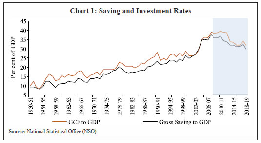 The gross domestic savings rate increased from 9.4 per cent in 1951-52 to 29.6 per cent in 2003-04 and further to a peak of 37.8 per cent in 2007-08 (Chart 1). Thereafter, the savings rate dropped to 30.1 per cent in 2018-19. At the disaggregated level, household savings and private corporate savings have shown a steady upward trend (Chart 2). Recent years have, however, seen a decline, largely reflected in household savings. Public sector savings declined after 1995-96, turning negative in 2000-01 and 2001-02 on account of an increase in the fiscal deficit. Public sector savings started improving after the introduction of the Fiscal Responsibility and Budget Management Act (FRBM) Act, 2003 (Reddy, 2008). 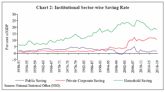 The private corporate savings rate improved from 4.3 per cent of GDP in 2003-04 to 12.2 per cent in 2007-08, a sharp uptick of around 8 percentage points. Thereafter, it stabilised at around 11 per cent. Similarly, private corporate investment rate increased from 8.6 per cent of GDP in 2003-04 to 21.0 per cent in 2007-08 (Chart 3). In the wake of the global financial crisis, private corporate investment fell sharply by about 7 percentage points and has lingered since then. The savings rate of the household sector, on the other hand, declined to 18.2 per cent in 2018-19 from 25.2 per cent in 2008-09, a drop of around 7 percentage points. The rate of gross capital formation had remained above the rate of gross domestic savings throughout the study period barring 2002-03 and 2003-04 when the current account was in surplus (Chart 4). In the post-global financial crisis period, the gap narrowed on the back of a sharper decline in the investment rate than the savings rate till 2010-11; since then, investment continued to weaken whereas savings showed a steady increase, resulting in lessening of the saving-investment gap.
III.2. Foreign Capital Flows into India3 The balance of payments accounting framework suggests that a country’s current and financial accounts have to be balanced ex-post, meaning that current account deficits (surpluses) will have to be matched by net capital inflows (outflows). It is the size of the current account deficit (CAD) that determines the absorptive capacity of foreign capital flows from a macroeconomic perspective. In other words, foreign savings only to the tune of CAD will ultimately add to investment. Large CADs, temporarily financed by net capital inflows, however, they are the source of imbalances over medium-term and lead to overheating and unsustainability. It is a useful yardstick to measure the contribution of capital flows to the domestic capital formation as it comprises flows such as external commercial borrowings (ECBs), foreign direct investments and forms of external assistance that may generally be earmarked for specific capital expenditure purposes. On the other hand, while Non-Resident Indian (NRI) deposits and portfolio flows may not directly contribute to capital formation; however, they may have an indirect effect on domestic capital formation rate through improvement in market liquidity and sentiments, and by serving to equilibrate the receipt–payment imbalance in the current account (Joshi, 2007). Starting from the time of independence till the 1980s, the external flows took place in the form of multilateral and bilateral concessional finance. The reform process was initiated after the balance of payment crisis in 1991. It included a swift transition to a market-determined exchange rate regime, dismantling of trade restrictions, a move towards current account convertibility and a gradual opening-up of the capital account (Mohan, 2008). In terms of the composition of capital flows, the policy reforms of 1991 intended to shift from debt creating flows to non-debt creating flows (Mohan, 2008). Consequent to the reforms, the Indian economy witnessed a high degree of capital inflows during the first half of the 2000s. The global financial crisis, 2008-09 led to an adverse situation characterised by global liquidity squeeze and increased risk aversion on the part of international portfolio investors. There were large capital portfolio outflows. While foreign direct investment (FDI) flows exhibited resilience, access to ECBs and trade credits was rendered somewhat difficult. In the post financial crisis period, different components of capital flows have behaved differently because of distinct factors. FDI, a stable component of foreign capital, declined during the crisis. Thereafter, it either remained stable or increased (Chart 5). In response to macroeconomic reforms undertaken following the exchange market pressure of 2013 and expectations of new structural reforms, foreign investments - both direct and portfolio flows - recorded substantial inflows. Net FDI inflows picked up sharply in response to initiatives that were geared towards a better business environment with policy certainty, viz., the ‘Make in India’ initiative, the Insolvency and Bankruptcy Code 2016, and impressive improvement in the Ease of Doing Business rankings. 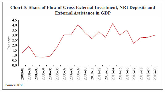 An important development in the post-financial crisis period is the lower ECB flows to India relative to the pre-crisis period. This can partly be attributed to the decline in corporate investment and more lately, easier domestic financial conditions which even led corporates to prepay ECBs. Therefore, it is worthwhile to revisit the association between aggregate savings and investment and examine the changes during the post-financial crisis period. Section IV
Data and Methodology IV.1. Data The empirical analysis in the paper is based on annual data for the period 1955-56 to 2018-19 extracted from ‘Handbook of Statistics on the Indian Economy’ published by the RBI. The nominal savings and investment figures are divided by nominal GDP at market prices at 2011-12 base. To ascertain the incremental impact of the changes that took place during the post-global financial crisis period, we undertake a separate analysis for the (sub-sample) period 1955-56 to 2007-08, and then for the full sample. ARDL model has been applied for the empirical estimation. IV.2. ARDL Model The total sample size in our estimation is 63, which is small and may give spurious results if estimated using a method which requires large sample size. Therefore, we apply the bounds test method of cointegration developed by Pesaran et al. (1999) and Pesaran et al. (2001), which is more efficient in the case of small and finite sample size. Additionally, the technique has the following advantages over other time series methods: (i) the model can be applied on data with a mix of stationary and non-stationary series; (ii) it provides unbiased long-run estimates; and (iii) it can provide both short and long-run relationship between variables along with the error correction process. Stationarity test is required only to ensure that variables are not integrated of order two or higher, as critical bound test values are not valid under these conditions. In the ARDL approach, we have established a long-run relationship among variables using a bound test. In the bounds test, the null hypothesis of no cointegration is tested against the alternative hypothesis that there is cointegration. Based on the comparison of computed F-statistic with the lower-bound (corresponding to I(0) series) and upper-bound critical value (corresponding to I(1) series), inferences can be drawn about the long-run relationship. If the computed F-statistic is higher than the upper bound critical value, the null hypothesis of no cointegration is rejected, signifying there is a long-run relationship between savings and investment. Once the long-run relationship is established, the next step is to estimate the long and the short-run coefficients of the cointegrated equation using the following error correction model (ECM):
where β is the long-run coefficient of saving-GDP ratio. The next section discusses the empirical findings. Section V
Empirical Findings We apply three methods to test the stationarity of the variables, i.e., Augmented Dickey-Fuller test (ADF, 1981), Phillips-Perron test (PP, 1988) and Kwiatkowski-Phillips-Schmidt-Shin test (KPSS, 1992). They all suggest that the variables are non-stationary in levels, but stationary in their first difference (Table 1). Based on stationarity tests, we apply the ARDL model to data for the sub-sample (1955-56 to 2007-08) and then to the full sample (1955-56 to 2018-19). Before discussing the ARDL results, it will be useful to look at the descriptive statistics (Table 2). The additional 11 observations (2008-09 to 2018-19) that distinguish the full sample from the sub-sample contain new information and provide some useful insights. The mean values of investment and saving rates are higher in the full sample. The corresponding average of saving-investment gap was lower for the full sample period. The volatility in the sub-sample period was also lower compared with that in the full sample period, mainly due to higher volatility in investment during the post-2007 period. | Table 1: Unit Root Test | | Test | Augmented Dickey-Fuller Test Statistic | Phillips-Perron Test Statistic | Kwiatkowski-Phillips-Schmidt-Shin Test Statistic | | Level | First Difference | Level | First Difference | Level | First Difference | | Investment Rate | -1.296 | -8.863*** | -1.238 | -8.943*** | 1.017 | 0.074*** | | Saving Rate | -0.888 | -8.022*** | -0.880 | -8.021*** | 1.012 | 0.088*** | | Note: ***: indicates significance at 1 per cent level. |
| Table 2: Descriptive Statistics | | Model | No. of Observations | Mean | Standard Deviation | Coefficient of Variation | Max | Min | | Sample:1955-56 to 2007-08 | | Investment to GDP Ratio | 53 | 21.8 | 6.3 | 28.9 | 39.1 | 12.7 | | Saving to GDP Ratio | 53 | 19.2 | 6.9 | 35.9 | 37.8 | 9.2 | | Saving-Investment Gap | 53 | -2.7 | 1.2 | -44.4 | 0.55 | -4.8 | | Sample:1955-56 to 2018-19 | | Investment to GDP Ratio | 64 | 24.2 | 7.9 | 32.6 | 39.8 | 12.7 | | Saving to GDP Ratio | 64 | 21.6 | 8.3 | 38.4 | 37.8 | 9.2 | | Saving-Investment Gap | 64 | -2.6 | 1.2 | -46.2 | 0.55 | -4.8 | The correlation between savings and investment rate was very high and statistically significant in both the samples, implying a steady co-movement over the years (Table 3). Furthermore, the correlation coefficient of the full sample is marginally higher than the sub-sample. Table 4 presents the findings from the ARDL bounds test for cointegration between domestic investment and domestic savings. For both the samples, F-statistic is higher than the upper bound critical value, confirming cointegration between variables and hence, a long-run relationship. The results of the estimated error-correction model are given in Table 5. The usual diagnostic and stability tests suggest the robustness of the estimates. Higher adjusted R-square indicates a good fit of the model. The null hypothesis of no serial correlation was accepted by the Breusch–Godfrey Serial Correlation Lagrange Multiplier (LM) test. Similarly, Breusch-Pagan-Godfrey heteroskedasticity test indicates acceptance of the null hypothesis of homoscedastic errors. The cumulative recursive residuals (CUSUM) and the cumulative sum of squares of recursive residuals (CUSUMQ) confirm the stability of the long-run coefficients in the ARDL model. | Table 3: Correlation between Savings and Investment | | Model | Coefficient | P-Value | | Sample:1955-56 to 2007-08 | 0.986 | 0.00 | | Sample:1955-56 to 2018-19 | 0.990 | 0.00 |
| Table 4: Bounds Test for Cointegration | | Model | F-Statistic | 99% lower bound | 99% upper bound | Inference | | Sample:1955-56 to 2007-08 | 8.60 | 6.84 | 7.84 | Cointegrated | | Sample:1955-56 to 2018-19 | 8.39 | 6.84 | 7.84 | Cointegrated | Table 5 shows long and short-run estimates of domestic investment and savings relationship along with the error correction term, which specifies the speed of adjustment if a deviation occurs from the long-run steady path. The long-run coefficient of saving is 0.90 which is statistically significant for the sub-sample period. The statistically significant coefficient increases to 0.94 for the full sample period when the post-financial crisis period is included. The higher magnitude of the coefficient points to a relatively higher association between saving and investment and less use of foreign savings. The outlier dummy used for the years 1976-77 and 1990-91 are statistically significant. The error correction term indicates that the short-run deviation from its steady-state path is corrected in two years. The adjustment was relatively quicker before the global-financial crisis. In the short-run also, savings play an important role in financing investment. | Table 5: Gross Domestic Savings and Investment: Error-Correction Results | | Variable | Sample: 1955-56 to 2007-08 | Sample: 1955-56 to 2018-19 | | Long-run | | Savings to GDP ratio | 0.90*** | 0.94*** | | Short-run | | Constant | 2.46*** | 1.87*** | | D (Savings to GDP ratio) | 0.94*** | 0.92*** | | Dum76 | -1.37** | -1.29** | | Dum90 | 1.80** | 1.63* | | Error-Correction Term | | ECR | -0.53*** | -0.47*** | | Diagnostic Tests | | Adjusted R-squared | 0.82 | 0.80 | | Breusch-Godfrey Serial Correlation LM Test | 0.31 | 0.11 | | Heteroskedasticity Test: Breusch-Pagan-Godfrey | 0.55 | 0.13 | | CUSUM | Stable | Stable | | CUSUM of Squares Test | Stable | Stable | | Note: ** and ***: indicates significance at 5 per cent and 1 per cent level, respectively. | The results suggest a comparatively lower association between saving and investment in the post-global financial crisis period. This implies a relatively lower use of foreign savings and a higher dependence on domestic savings. The growth in real fixed investment in the post-global financial crisis period turned to a single digit except 2010-11 and 2011-12 and much lower in 2008-09 and 2012-13 to 2015-16. This slowdown was largely due to private corporate investment. Out of 6.3 percentage points decline in the overall investment rate (investment as per cent to GDP) during 2007-08 to 2015-16, private investment accounts for 5 percentage points (GOI, 2017). India’s investment slowdown is a balance sheet related slowdown (GOI, 2017). Many companies have had to curtail their investments because their finances are stressed, as the investments made during the boom period have not generated enough revenues to allow them to service the debts that they have incurred. The decline in domestic saving was led equally by household and public sector saving. The fall in the former was on account of physical saving. The private corporate saving, on the other hand, has increased steadily. Section VI
Robustness Check A robustness check of results presented in the previous section is performed by applying the same ARDL model to quarterly saving and investment data. These data are, however, not readily available. The investment includes fixed investment, change in stocks, valuables and errors and omissions.4 The data for errors and omissions are available at an annual frequency; the quarterly gross capital formation data do not include this component. Similarly, savings data are available only at an annual frequency. The above limitations suggest that one must construct quarterly saving and investment data in order to run the ARDL model. From the investment side, we have used Denton method5 of frequency conversion to extract quarterly errors and omissions data from annual figures. After that, quarterly investment is added to quarterly current account balance to arrive at domestic savings. The data are shown in Chart 6a and 6b. 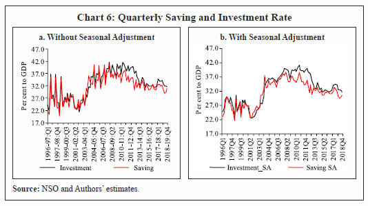 For the empirical exercise, we follow the approach of Bayoumi (1990) and Abbott and Vita (2003), that the use of total investment (which includes inventories as well as business fixed investment) may lead to spurious correlations with savings that reflect endogenous behaviour by private agents. Therefore, we have used gross fixed capital formation. After the construction of data, the long-run relationship between saving and investment is tested. Both variables are seasonally adjusted and used as a per cent to GDP. They are non-stationary in levels but stationary in first difference. | Table 6: Bound Tests for Cointegration | | Model | Time Period | F-Statistic | 99% lower bound | 99% upper bound | Inference | | 1 | 1996-97: Q1 to 2008-09: Q4 | 9.32 | 6.84 | 7.84 | Cointegrated | | 2 | 1996-97: Q1 to 2018-19: Q4 | 15.47 | 6.84 | 7.84 | Cointegrated | Unlike annual data, quarterly frequency allows more number of observations. We have applied ARDL model to the sub-sample from 1996-97: Q1 to global financial crisis year i.e. 2008-09 and full sample (including post-global financial crisis period). Table 6 indicates the cointegrating relationship between saving and investment in both samples, as F-statistics are higher than their respective lower and upper critical bound values. Table 7 presents the error-correction results of the two samples. The model satisfied all the diagnostic criteria. The error-correction term is negative and statistically significant. The saving coefficients in both the samples are very close to the coefficients in the annual estimated results. Though both coefficients are closer to one, in full sample they are relatively higher than the sub-sample, indicating a relatively higher association between the variables and comparatively lower dependence on foreign saving. | Table 7: Gross Domestic Savings and Investment: Error-Correction Results | | Variable | Sample: 1996-97:Q1 to 2008-09:Q4 | Sample: 1996-97:Q1 to 2018-19Q4 | | 1 | 2 | 3 | | Long-run | | Savings to GDP ratio | 0.91*** | 0.94*** | | Short-run | | Constant | 0.33*** | 0.09 | | D(Investment to GDP ratio(-1)) | - | -0.05 | | D(Investment to GDP ratio(-2)) | - | 0.09 | | D(Investment to GDP ratio(-3)) | - | 0.21** | | Dum2006Q3 | 1.24** | -2.92*** | | Dum2010Q1 | - | 1.37** | | Error-Correction Term | | ECR | -0.17*** | -0.17*** | | Diagnostic Tests | | Adjusted R-squared | 0.34 | 0.49 | | Breusch-Godfrey Serial Correlation LM Test | 0.89 | 0.10 | | Heteroskedasticity Test: Breusch-Pagan-Godfrey | 0.78 | 0.77 | | CUSUM | Stable | Stable | | CUSUM of Squares Test | Stable | Stable | | Note: ** and ***: indicates significance at 5 per cent and 1 per cent level, respectively. | Section VII
Is India an outlier? Previous sections demonstrate that saving and investment rates in India have displayed a high degree of co-movement except for a brief period. This co-movement has existed despite progressive liberalisation of the capital account. As discussed in Section II, this puzzle is not unique to India. In fact, in most advanced economies the saving-investment correlations are high. In a recent study analysing cross-country experience, David, Gonçalves and Werner (2020) concluded that frictions in global financial markets are the main explanation for the high positive correlation between saving and investment. This is more pronounced in the case of emerging market economies vis-à-vis advanced economies. Other explanations provided in the literature are global productivity shocks and international trading cost (Glick and Rogoff, 1995; Obstfeld and Rogoff, 2000). However, during the post-GFC period, India didn’t witness a decline in productivity (RBI, 2019) and rise in trading cost. Trading cost, measured by transportation cost, has continued its downward trend6. Therefore, frictions emanating from global financial crises could be a possible explanation for high saving investment correlation, reflecting risk aversion among economic agents. This section analyses the changes in cross-country investment and saving after various crises and draws inferences to examine whether India is an outlier. Accordingly, we analysed movements in saving rate, investment rate and saving-investment gap of crisis-affected economies, starting from the Mexican peso crisis (Table 8). The timing of crises and crisis-affected economies are decided based on a literature survey. For ascertaining a change in saving and investment behaviour of crisis-affected economies, we compare their average saving and investment rates before and after the crises year. We use a five-year average of pre-crises and post-crises saving and investment rates for each affected economy. Accordingly, we have 21 economies with different crisis episodes. | Table 8: National Saving-Investment of Crisis-affected Economies – Pre- and Post-crises | | (Per cent) | | Crisis | Economy | Investment | Saving | | Pre-crisis | Post-crisis | Pre-crisis | Post-crisis | | Mexican peso crisis (Jan 1995) | Mexico | 23.6 | 22.6 | 18.9 | 22.9 | | Brazil | 20.5 | 17.6 | 19.5 | 12.3 | | Russian flu (August 1998) | Russia | 22.3 | 20.4 | 25.2 | 30.8 | | East Asian currency crisis (July 1997) | Indonesia | 30.0 | 22.1 | 28.8 | 22.4 | | South Korea | 38.3 | 31.7 | 37.1 | 34.1 | | Thailand | 40.0 | 22.1 | 34.9 | 29.9 | | Hong Kong | 31.8 | 25.3 | NA | 31.4 | | Malaysia | 41.7 | 24.6 | 35.6 | 35.8 | | Philippines | 23.9 | 18.5 | 19.1 | 33.7 | | Global financial crisis (2008) | USA | 26.6 | 27.4 | 18.1 | 16.1 | | European debt crisis (2009-2011) | Greece | 22.6 | 11.6 | 9.9 | 8.6 | | Portugal | 22.3 | 15.4 | 11.9 | 14.7 | | Ireland | 24.6 | 21.7 | 20.1 | 21.3 | | Spain | 27.0 | 18.1 | 20.0 | 19.2 | | Cyprus | 25.0 | 13.9 | 14.8 | 12.4 | | Taper tantrum (May 2013) | Brazil | 21.1 | 15.5 | 17.7 | 14.0 | | India | 39.2 | 31.8 | 35.7 | 32.5 | | Indonesia | 31.9 | 34.1 | 31.1 | 30.5 | | South Africa | 20.6 | 19.8 | 17.1 | 16.0 | | Turkey | 27.7 | 29.2 | 22.4 | 24.5 | NA: Not available,
Note: List of economies is prepared on the basis of literature and contemporary media reports.
Source: Authors’ calculation based on World Bank data. | It can be observed that after the crisis, investment rate of all countries, except those of the USA (GFC), Indonesia and Turkey (after 2013), declined significantly (Table 8). Saving rate also declined after the crisis, though at a comparatively moderate pace than the decline in investment rate. In fact, many economies were able to increase their saving rate after the crisis. The result of this asymmetric behaviour of economies gets reflected ultimately in their saving-investment gap, which records a sharp decline in the post-crises period vis-à-vis pre-crises period (Chart 7). Out of 21 crisis-affected country episodes, only the USA (2007-08), Brazil (1994) and Indonesia (2013) recorded a higher saving-investment gap post-crisis, while all others recorded narrower gaps. This experience reinforces the role of frictions in global financial markets, which manifest from time to time in crises, leading to a higher correlation between domestic saving and investment rate. Thus, the observed saving-investment relationship in India is not an exception. Section VIII
Conclusion The capital account in India has been facilitating greater cross-border movement of capital. This paper examines whether the dependence of domestic investment on domestic savings has declined following greater access to availability of foreign capital. The empirical results confirm a long-run relationship between domestic savings and investment. A comparison of the long-run coefficients for the full sample period (1955-56 to 2018-19) with that for the sub-sample period (1955-56 to 2007-08) indicates a relatively higher degree of association between domestic savings and investment. This, in turn, suggests a reduced role of foreign saving in financing investment activity after the global financial crisis of 2007-09. This largely reflects moderation in private corporate investment rate in the post-global financial crisis period. The error correction term indicates that in the event of short-run deviations from the steady state relationship between savings and investment, the restoration of equilibrium takes about two years. Furthermore, the adjustment was relatively quicker before the global financial crisis. An analysis of episodes of financial crises behaviour of several economies reveals that in the aftermath of one crisis, there is a decline in saving-investment gap, thereby, emphasising the role of frictions in global financial markets, leading to a higher correlation between domestic saving and investment rate. Thus, the case of India is not an exception. Going forward, as physical capital formation revives, it should also be backed by a commensurate rise in domestic savings for sustained long-run growth. At the same time, it is important to enhance the efficiency of domestic financial system to improve the allocation of resources to the most productive sectors.
References Abbott, A.J. & Vita, G.D. (2003). Another Piece in the Feldstein-Horioka Puzzle. Scottish Journal of Political Economy. Vol. 50 (1). Bayoumi, T. (1990). Saving–investment correlations: immobile capital, government policy or endogenous behavior. IMF Staff Papers, 37, pp. 360–87. David A.C., Gonçalves, C. E., & Werner, A. (2020). Reexamining the National Savings-Investment Nexus Across Time and Countries. IMF Working Paper,124. Denton, F. T. (1970). Quadratic minimization procedures for adjusting monthly or quarterly time series to independent annual totals, McMaster University Department of Economics, Working Paper 70-01. Dickey, D. A., & Fuller, W. A. (1981). Likelihood ratio statistics for autoregressive time series with a unit root. Econometrica: journal of the Econometric Society, 1057-1072. Ekong, C. N. & Onye, K. U. (2015). International Capital Mobility and Saving-Investment Nexus in Nigeria: Revisiting Feldstein-Horioka Hypothesis. Science Journal of Business and Management, 3 (4), 116-126. Feldstein, M. & Horioka C. (1980). Domestic Saving and International Capital Flows. Economic Journal, 90 (358), 314-329. Glick, R. & Rogoff, K. (1995). Global versus Country-Specific Productivity Shocks and the Current Account. Journal of Monetary Economics, 35 Government of India (GoI) (2017). ‘Chapter II:The Economic Vision for Precocious, Cleavaged India’, Economic Survey 2016–17, I, 38–53 Government of India (GoI) (2018). ‘Chapter III: Investment and Saving Slowdowns and Recoveries: Cross-Country Insights for India’, Economic Survey 2017–18, I, 43–54 Iorio, Francessca De & Fachin, S. (2011). A Panel Co-integration Study of the Long Run Relation between Saving and Investment in the OECD Economies 1970-2007. MRPA Paper, No. 25873. Jangili, R. (2011). Causal relationship between saving, investment and economic growth for India? What does the relation imply? RBI Occasional Paper, 32 (1). Joshi, H. (2007). The Role of Domestic Saving and Foreign Capital Flows in Capital Formation in India. RBI Occasional Papers, 28 (3). Kaur, H. & Sarin, V. (2019). The Saving-Investment Co-integration Across East Asian Countries: Evidence from the ARDL Bound Approach. Global Business Review, 1-9 Khundrakpam, Jeevan K. & Ranjan, R. (2010). Saving-Investment Nexus and International Capital Mobility in India: Revisiting Feldstein-Heroic Hypothesis. Indian Economic Review, 45(1), 49-66. Kwiatkowski, D, Phillips, P.C.B., Schmidt, P., & Shin, Y. (1992). Testing the Null Hypothesis of Stationarity against the alternative of a unit root: How sure are we that economic time series have an unit root? Journal of Econometrics, 54(1-3). Mohan, R. (2008). Capital Flows to India, Manuscript, Reserve Bank of India. Paper presented at annual meeting of Deputy Governors at BIS, February 2008. Obstfeld, M. & Rogoff, K., 2000. The Six Major Puzzles in International Macroeconomics: Is There a Common Cause? NBER Working Paper. Pesaran, M. H., Shin, Y. &Smith, R. J. (1999). Bounds Testing Approaches to the Analysis of Long-Run Relationships. DAE Working Paper No. 9907, Department of Applied Economics, University of Cambridge. Pesaran, M. H., Shin, Y., & Smith, R. J. (2001). Bounds testing approaches to the analysis of level relationships. Journal of applied econometrics, 16(3), 289-326. Phillips, P. C. B. & Perron, P. (1988). Testing for a Unit Root in Time Series Regression. Biometrika, 75 (2), 335–346 Prakash, A., Shukla, A.K., Ekka, A.P., Priyadarshi, K. & Bhowmick, C. (2019). Financial Stocks and Flows of the Indian Economy 2011-12 to 2017-18, RBI Bulletin, 73(7), 41–57. Rashid, Abdule & Jehan, Zanaib. (2013). Derivation of Quarterly GDP, Investment Spending, and Government Expenditure Figures from Annual Data: The Case of Pakistan. MPRA, Paper No 46937. Reserve Bank of India. (2015). Is India ready for full Capital Account Convertibility?, Address by Shri G Padmanabhan, Executive Director at MSNM Besant Institute of PG Management Studies Mangalore on May 16, 2015. Reddy, Y. V. (2008). Fiscal Policy and Economic Reforms. NIPFP Working Paper, 2008-53. Reserve Bank of India (RBI). (2019). Reserve Bank of India Annual Report 2018–19, Reserve Bank of India, Mumbai. Singh, T. (2008). “Testing the Saving-Investment Correlations in India: An Evidence from Single Equation and System Estimators. Economic Modelling, 25, 1064-1079. Sinha, D. & Sinha, T. (1998). An Exploration of the Long-Run Relationship Between Savings and Investment in the Developing Economies: A Tale of Latin American Countries. Journal of Post Keynesian Economics, 20, 435-443. Srivastava, V.K, Shukla, A.K., Seth, B. & Priyadarshi, K. (2018). Statistical Discrepancies in GDP Data: Evidence from India, RBI Bulletin, 72(2), 31–48. Verma, R. (2007). Savings, Investment and Growth in India: An Application of the ARDL Bounds Testing Approach. South Asia Economic Journal, 8(1), 87-98. Vuyyuri, S. & Sakalya, V. S. (2005). Savings and Investment in India, 1970-2002: A Cointegration Approach. Applied Econometrics and International Development, 5(1). Yadav, I. S, Goyari, P. & Mishra, R.K. (2018). Saving, Investment and Growth in India: Evidence from Co-integration and Causality Tests. Economic Alternatives, 1, pp 55-68.
|