Saurabh Ghosh, Sujata Kundu and Archana Dilip* Received on: June 28, 2021
Accepted on: September 23, 2021 The paper attempts to analyse the causal impact of natural disasters on output growth, agricultural productivity, inflation, tourism, fiscal parameters, and the cost of borrowing of Indian coastal states. It considers five states along the western coastline, i.e., Gujarat, Maharashtra, Goa, Karnataka and Kerala, and four states along the eastern coastline i.e., West Bengal, Odisha, Andhra Pradesh and Tamil Nadu and their eight neighbouring inland states in order to assess the impact. Difference-in-difference regression results covering the sample period 2011-12 to 2019-20 indicate that natural disasters lower output growth, raise inflation and dampen tourist arrivals, while borrowing costs largely remain unaffected. Some of these adverse effects also persist in the subsequent years. Eastern coastal states appear to have learnt and adapted better, given their long history of dealing with fierce natural disasters. For enhancing resilience of those directly affected, it is necessary to strengthen disaster management capabilities, incentivise green projects, undertake scenario analyses for effective policy preparedness and promote green finance. JEL Classification: C33, E31, O13, Q54 Keywords: Green swan, panel data, difference-in-difference, green finance Introduction Green swans1 or climate black swans have many features of typical black swans, such as their unexpected and rare nature of occurrences, wide-ranging impact and also that they can be explained only after the event has occurred. The Bank for International Settlements (BIS) defines two sets of risks associated with climate change that are of particular concern, viz., physical risks and transition risks (BIS, 2021a). Physical risks arise from climate and weather related catastrophe events, such as droughts, floods, storms and rise in sea levels which cause damages to property, land and infrastructure. Apart from these direct impacts, physical risks could emerge indirectly through ensuing events such as disruption of global supply chains and lower productivity of agriculture and consequently, inflation. The transition risks, on the other hand, refer to the financial risks which emanate from the process of adjustment towards a lower carbon economy. While this transition creates opportunities for innovation, investment and potential green growth, changes in climate policy, technology or market sentiment could lead to re-pricing of a range of assets and may turn out to be crucial for the soundness of financial firms. Climate-related risks are generally fat-tailed distributions, with both physical and transition risks being characterised by deep uncertainty and non-linearity. According to Weitzman (2009), their chances of occurrence are not reflected in past data, but there is a possibility of extreme values. Green swans are different from black swans in three aspects, viz., certainty, intensity and complexity (Bolton et al., 2020). Although the impact of climate change is uncertain, there is a high degree of certainty that some combination of physical and transition risks will materialise in future (NGFS, 2019). Central banks are increasingly focusing on the risks from climate change for the economy and financial system. Since the issue is multifaceted, it requires calibrated policy responses, even within a central bank, as climate change and related policies could have a potential impact on key economic indicators relevant to monetary policy. These include output growth, inflation, investment, and the cost of funds. Given the degree of interconnectedness in the economy and the financial system, it is important to assess both the direct impact of physical and transition risks and the indirect and second-round effects. This implies accounting for exposures along the whole production chain, the transmission of shocks through financial linkages and feedback loops between the macroeconomy and the financial sector. This poses challenges for assessing the channels that could affect the economy and financial system. There is also considerable uncertainty about future developments in policy, technology, natural environment and other factors related to climate change. India was placed at the seventh position in the list of most affected countries in terms of exposure and vulnerability to extreme weather events in 2019 after Mozambique, Zimbabwe, the Bahamas, Japan, Malawi and Afghanistan (Global Climate Risk Index, developed by Germanwatch), though in terms of long-term average score for the period from 2000 to 2019, India did not feature in the ten worst affected economies. An analysis of major weather-related events in the Indian context since 1901 reveals significant changes in climatic patterns in the past two decades with increased volatility in precipitation patterns relative to the long period average (LPA) and rising annual average temperature levels (Dilip and Kundu, 2020). The dynamics of the South-west Monsoon (SWM) have also changed over the years with the withdrawal dates of monsoon showing a delay which has a significant impact on the cropping seasons/patterns. Importantly, in India, growth and inflation outlook continue to be heavily influenced by the amount of rainfall and its distribution during the SWM season (June-September). Moreover, along with the gradual changes in temperature and rainfall patterns, the incidence of extreme weather events, such as excessive rainfall often leading to floods, severe temperature fluctuations (e.g., heat waves and cold waves) and cyclones are being witnessed with rising frequency and intensity. Unseasonal rainfall, which heavily impacts the outlook on food inflation has also been a rising concern in recent years. The regional spread of these extreme weather events shows that some of the major agricultural states (either food grain or cash crop producers) are the most affected ones (particularly, Andhra Pradesh, Odisha, West Bengal, Gujarat, Maharashtra and Madhya Pradesh). With this background, it would be interesting to study the impact of extreme weather events, in particular cyclones, floods and droughts, that have become a regular feature in India on some of the crucial macro, fiscal and financial indicators. In the Indian context, we found limited literature that analyses the causal impact of these green swan events with an appropriate identification strategy. We, therefore, attempt to bridge this gap by considering the Indian coastal states that are directly affected by these extreme events and compare the economic parameters of these states with a control set of neighbouring inland states. This research design, using the difference-in-difference (D-i-D) panel data based econometric approach, evaluates the causal impact of green swan events on income, agricultural yields, tourism, inflation, fiscal parameters and cost of borrowings. The findings suggest that natural calamities cause a decline in economic growth and have a lingering impact on income growth; a decline in the yields of vegetables and fruits and tourist arrivals; a rise in inflation; and that the spillover impact of such extreme events persists in the subsequent years. The paper is structured as follows. Section II provides a brief review of literature related to the impact of climate-related risks on the economy and the available mitigation options. The stylised facts with respect to the changing climate pattern witnessed in India over the years, with a particular focus on coastal states are presented in Section III. Section IV describes the data used in the empirical analysis. Section V presents the D-i-D research design used to study the causal effects of natural calamities on an array of macro variables in India comprising Gross State Domestic Product (GSDP), agricultural yields, inflation, fiscal and financial variables. The empirical findings are also presented in Section V. Section VI provides an overview of the green finance policy and the mitigation policy recommendations. Concluding remarks are provided in Section VII. Section II
Review of Literature Studying the impact of climate change on the economy is an age-old area of interest for economists. Some of the earliest works in this sphere date back to as far as Fisher (1925), which examined the effects of rainfall on the yields of wheat. Climate change can be considered as an exogenous factor that drives or influences economic activity and macroeconomic outcomes. In the recent times, with climate change and its associated extreme weather events becoming a major challenge globally, questions concerning weather conditions and their impact on the macroeconomy are increasingly gaining the spotlight. Across the literature reviewed, many broad themes emerge and most studies have focussed on the range of channels through which extreme weather events affect an economy. The most recent studies including Batten et al. (2020) and BIS (2021a; 2021b) have thrown light on the major climate-related risks and their transmission channels. BIS (2021b) provided an overview of the conceptual issues related to climate-related financial risk measurement, methodologies and practical implementation by banks and supervisors. The report addressed the need for sufficiently granular and forward-looking measurement methodologies to capture the unique features of climate-related financial risks. BIS (2021a) explored how climate-related risk drivers, both physical and transition risks, impact the banking system through microeconomic and macroeconomic transmission channels. While the microeconomic transmission channels include the causal chains by which climate risk drivers affect banks’ individual counterparties, the macroeconomic transmission channels refer to the mechanisms by which climate risk drivers affect macroeconomic factors like labour productivity and economic growth. These channels also capture the effects of market variables like risk-free interest rates, inflation, and foreign exchange rates. The report also highlighted the variation in economic and financial market impacts of physical and transition risks based on geography, sector and economic and financial system development. The geographical heterogeneity is driven by factors including differences in the likelihood and severity of climate risk drivers, structural differences in economies and markets that affect the importance of various transmission channels and differences in financial systems that impact banks’ exposures to climate-related risks. Furthermore, Batten et al. (2020) reviewed the channels through which climate risks could affect central banks’ monetary policy objectives and the possible policy responses. The paper also discussed various approaches that aim to incorporate climate change in central bank macro-modelling frameworks. Secondly, there are various studies that have analysed the impact of different dimensions of climate change on different aspects of an economy (Dell et al., 2014). Under this category, studies may be further divided into: (i) studies that consider many countries simultaneously and; (ii) studies that concentrate upon a particular economy. The popular studies in the former category include Kahn et al. (2019) that considers 174 countries, and Feyen et al. (2020) that considers many countries from East Asia and the Pacific (EAP), Europe and Central Asia (EAC), Latin America and Caribbean (LAC), Middle East and North Africa (MENA), South Asia (SA) and Sub-Saharan Africa (SSA). In order to study the long-term impact of climate change on economic output across countries, Kahn et al. (2019) used a panel dataset of 174 countries for the period from 1960 to 2014 and found that per capita real output growth is adversely affected by persistent deviations in temperature from its historical norm. Feyen et al. (2020) studied the inter-relation between macro-financial and climate-related risks and highlighted that many countries face the double-jeopardy of simultaneous elevation of both risks. The authors highlighted that the climate changes and consequent macroeconomic changes will have significant impact on the balance sheets of key economic entities. Transition risks are likely to be high for countries that generate a significant share of public revenue from carbon-intensive industries. On the central banking and monetary front, their research indicated that the interactions between climate change, climate policies, and monetary conditions and management are in a relatively nascent stage. However, climate‐related financial risks may weaken financial sector balance sheets and induce or amplify macro-financial risks as physical impacts of climate change can lead to heightened operational, credit, market, and liquidity risks for banks. The paper suggested that banks need to build capacity and integrate climate factors into all aspects of their operations. It also suggested a slew of policy measures and concluded that the implementation of climate mitigation and adaptation measures could be a significant driver of economic growth. Several studies have looked at the influence of changing weather realisations on agricultural and industrial output, labour productivity, demand for utilities like energy and health services and overall economic growth by concentrating on an individual economy. Most of the studies under this category pertain to developed economies. For instance, Bloesch and Gourio (2015), using a panel of states of the United States (US), found evidence supporting the view that weather conditions impact economic activity, particularly in sectors such as utilities, construction, hospitality and retail, even though the impact could be short-lived. Another study using a panel regression framework with GSDP and average seasonal temperature data for US states found that a rise in summer temperature has an adverse effect on GSDP growth, while a rise in the average temperature during the autumn season positively affects GSDP growth, although the impact is weaker and less robust (Colacito et al., 2018). A study by Tokunaga et al. (2015) identified the impact of global-warming-induced climate change on Japan’s agricultural production using both static (using a function for agricultural products incorporating labour, temperature, solar radiation and precipitation) and dynamic (using a production function for agricultural products incorporating labour, one-period lagged output and the three weather variables indicated above) panel data models on a cross-section of eight regions in Japan for the period 1995-2006. The paper concluded that an increase of 1oC in mean annual temperature results in a fall of rice production by 5.8 per cent and 3.9 per cent in the short-term and long-term, respectively, while in the case of vegetables, production falls by 5.0 per cent and 8.6 per cent in the short-term and long-term, respectively. Lastly, the emerging research has considered other important channels or dimensions like cross-border effects. While studying the cross-border spillovers of physical climate risks through trade and supply chain linkages, Feng and Li (2021) observed that globalisation increased the similarity of countries’ global climate risk exposures. On the basis of historical data from 1970-2018, the paper argued that exposures to foreign climate-related disasters among important trade partner countries could have negative effects on the stock-market valuation of the aggregate market and for the tradable sectors in the home-country. The paper further observed that the extent of financial stability implications depends on country-specific factors like the size of tradable sectors to the overall economy and exposure of domestic banks to tradable sectors. In the Indian context, the studies are generally based on quantifying physical risks and analysing the impact on different aspects of macro economy. Using a pooled mean group regression technique on state-level panel data, Parida and Dash (2019) found that floods negatively impact per capita GSDP in the long run. Studies focusing specifically on the impact of climate-related risks on the agriculture sector pointed out the adverse impact of weather-related events on crop yields. For example, Barve et al. (2019) showed that both rainfall and temperature-related unfavourable shocks adversely affect rice yields. Another paper by Madhumitha et al. (2021), studying the impact of adverse rainfall events in the agriculture sector, suggested that crop diversification could be useful towards mitigating climate-related challenges and risks in the agriculture sector particularly in areas that lack specialisation in a particular crop or are lesser advanced in terms of irrigation facilities. However, the paper also indicated that the method may not provide positive results during extreme drought situations. Empirical findings based on pair-wise Granger-causality tests using annual data (1960-2014) in the Indian context, provided in Dilip and Kundu (2020), showed that economic activity measured by Gross DomesticProduct (GDP) per capita causes carbon dioxide (CO2) emissions, which in turn causes an increase in average temperature. Moreover, the results also indicated the existence of a bi-directional causality between temperature and GDP per capita. With respect to rainfall, the findings showed that rainfall affects the availability of gross irrigated area, which in turn affects agricultural yield (output and/or sown area). Further, it was noted that rainfall deviation is associated with food inflation (particularly inflation in vegetables and fruits), and the impact generally lasts for 5-6 months (Dilip and Kundu, 2020). An increase in the inflation of vegetables and fruits may significantly distort the overall food inflation path as these comprise a significant share of the food basket. The paper also highlighted through empirical analysis that weather conditions have a significant impact on some of the key indicators of economic activity like Purchasing Managers Index (PMI), Index of Industrial Production (IIP), demand for electricity, trade, tourist arrivals, and tractor and automobile sales. Although there is limited literature on transition risks in the Indian setup, Agarwal (2021) highlighted India’s path towards climate change objectives asratified in the Paris Agreement (PA)2. The paper cited the estimates of Climate Action Tracker to argue that India will comfortably surpass the targets set in the PA. The paper also pointed out that India is currently at a developmental stage (although emitting lesser than other countries when they were at a similar stage) and emissions would increase with increasing per capita GDP. However, since emissions and GDP per capita have an inverted U-shaped relationship, emissions are expected to decline after a peak. Further, the author mentioned that the vulnerable groups of the population may be protected while transitioning to carbon neutrality. The author cited research done in this area and inferred that carbon taxes may be used to finance cash transfers to poorer households. Thus, this kind of policy may have a distributional impact on the population of a country. Finally, in line with the existing global literature, the studies in the Indian context have also reviewed and recommended mitigation policies including green finance policies. Green finance has become a public policy priority all over the world. As noted by Ghosh et al. (2021), India has pushed forward green finance in relevant sectors in line with the global practices. Green bonds have constituted around 0.7 per cent of all the bonds issued in India since 2018, and the combined outstanding bank lending (excluding personal loans) by the public sector and private sector banks to the non-conventional energy is around 7 per cent of the outstanding bank credit into the utility sector (electricity, gas and water supply), as on March 2019. Ghosh et al. (2021) highlighted that most of the green bonds in India are issued bythe public-sector units3 or corporates with better financial health. Although the value of green bonds issued in India since 2018 has constituted a very small portion of the total bond issuance, India has maintained a favourable position as compared to several advanced and emerging market economies (EMEs). Two sectors that account for a large portion of the fossil fuel consumption in India are power generation and automobile industry. However, the share of automobile production in the aggregate bank credit is much smaller, at only 1.2 per cent (Ghosh et al., 2021). Both Ghosh et al. (2021) and Dilip and Kundu (2020) emphasised on the importance of awareness creation as the first step, which would be the prime responsibility of the governing bodies. There is a paucity of data for assessing the awareness regarding green finance and sustainable development from conventional sources (including statutory organisations, central banks). In this regard, Google Trends can be a powerful tool for understanding the dynamics of Google searches made in different locations at different points in time. Evidence based on Google Trends suggests an increase in awareness about green finance and its role in sustainable economic development (Ghosh et al., 2021). Section III
Stylised Facts The global phenomenon of climate change and the associated extreme weather events have emerged as key risks to the macroeconomic outlook of both developed economies and EMEs. Extreme weather events may be classified into four different types: geophysical (avalanche, landslides, earthquakes, volcanic eruptions); hydrological (floods, tsunami); meteorological (cyclones, droughts, heat waves, cold waves, thunderstorms, tornadoes); and climatological (arising from change in temperature and precipitationpatterns).4 III.1 Losses due to Natural Disasters In terms of damage to infrastructure, crops and livelihood, floods are the costliest, causing 63 per cent of damage, followed by cyclones (19 per cent), earthquakes (10 per cent) and droughts (5 per cent). In terms of human casualties in India, earthquake is the most lethal with 33 per cent of casualties, followed by floods (32 per cent), cyclones (32 per cent) and landslides (2 per cent) (World Bank, 2012). In 2020, India was ranked third after China and the US in recording the highest number of natural disasters over the last 20 years (UN, 2020). In the demographic front, globally, deaths caused by natural disasters stood at around 0.1 per cent on an average in the previous three decades (1990-2017), while in the case of India it was 0.04 per cent. Importantly, over the years, the percentage of deaths owing to natural calamities has fallen considerably on account of technological advances and improved early warning systems, large-scale government initiatives with regard to relief measures and pro-active disaster management policies (Chart 1a). However, natural calamities take a huge toll on the overall macroeconomic outcomes. Globally, economic loss due to natural calamities during the past three decades has ranged from 0.12 per cent to 0.50 per cent of world GDP (Chart 1b). III.2 Change in Climatological Pattern in India Change in overall climatic conditions has become increasingly visible in India. While annual average temperature has recorded a steady rise over the years, annual average rainfall shows a sharp decline (Chart 2a). Further, annual maximum temperature has witnessed a steep increase during the past two decades (Chart 2b).
III.3 Extreme Weather Events in the Indian Coastal States: Frequency and Intensity Based on the frequency of occurrence of extreme weather events in the recent times, it can be seen that the coastal states in India are affected mainly by cyclones, floods, droughts and rising sea levels. III.3.1 Cyclones Twelve decades of data (1901-2020) on cyclonic storms reveal that over the years, the frequency of severe cyclonic storms (intensity: ≥ 48 knots) has increased in India (Table 1). Further, the distribution of cyclones across the Bay of Bengal and the Arabian Sea show that there is a sharp jump in the occurrence of cyclonic storms over the Arabian Sea, which is in sharp contrast to the historical pattern. The pattern in the recent two decades (2001-2020) reveals that the average number of cyclones in the Arabian Sea equalled that of the Bay of Bengal, which is two cyclones per year. Historically, this number has been lower in the Arabian Sea as compared to that in Bay of Bengal. Further, a state-wise distribution of severe cyclones reveals that the number of cyclones that occurred in the states of Odisha, Andhra Pradesh and Tamil Nadu in the eastern coast of India during 1961-2020 was much higher than that during 1901-1960 (Chart 3a). Additionally, in the west coast, the incidence of severe cyclonic storms in Gujarat increased significantly during 1961-2020 as compared to Maharashtra and Goa. With regard to the intensity of severe cyclonic storms (SCS), the India Meteorological Department (IMD) classifies severe cyclones into the following four categories: severe cyclonic storms (SCS: 48-63 knots), very severe cyclonic storms (VSCS: 64-89 knots), extremely severe cyclonic storms (ESCS: 90-119 knots) and super cyclonic storms (SuCS ≥ 120 knots). Data available for the period from 1965 to 2020 show that out of the eight super cyclonic storms that occurred during this period over the north Indian Ocean, three of them (i.e., 38 per cent) occurred during 2001-2020 (Chart 3b). | Table 1: Frequency and Intensity of Cyclones | | Period | Number of Cyclones | Per cent | Average per Year | | Cyclones (>=34 knots)5 | | | Bay of Bengal | Arabian Sea | Total | Bay of Bengal | Arabian Sea | Bay of Bengal | Arabian Sea | | | (1) | (2) | (3) | (4) | (5) | (6) | (7) | | Full Period: 1901-2020 | 474 | 126 | 600 | 79 | 21 | 4 | 1 | | Sub-period: 1901-1960 | 267 | 53 | 320 | 83 | 17 | 4 | 1 | | Sub-period: 1961-2020 | 207 | 73 | 280 | 74 | 26 | 3 | 1 | | Sub-period: 2001-2020 | 49 | 32 | 81 | 60 | 40 | 2 | 2 | | | Severe Cyclones (>= 48 knots) | | Full Period: 1901-2020 | 219 | 78 | 297 | 74 | 26 | 2 | 1 | | Sub-period: 1901-1960 | 90 | 30 | 120 | 75 | 25 | 2 | 1 | | Sub-period: 1961-2020 | 129 | 48 | 177 | 73 | 27 | 2 | 1 | | Sub-period: 2001-2020 | 26 | 22 | 48 | 54 | 46 | 1 | 1 | | Source: India Meteorological Department (IMD); and Authors’ calculations. |
III.3.2 Droughts and Floods Hydroclimatic extremes such as droughts and floods are characteristic features of any monsoonal landscape. Droughts over India are typically associated with prolonged periods of abnormally low monsoon rainfall that can last over a season or longer and may also affect several states at a time (Sikka, 1999). The overall decrease in annual rainfall in India as shown previously in Chart 2a is primarily a result of a decline in the rainfall received during the SWM season. India receives around 75 per cent of its annual rainfall during these four months of the year. However, data reveal that over the years, average monsoon departures from the LPA rainfall have largely tended to be below normal (Chart 4). This trend is also reflected in the incidence and intensity of droughts in the country. The number of droughts that occurred in India during 1961-2020 stood at 14 as compared to eight during 1901-1960 (Table 2). Further, in terms of drought intensity, years with severe droughts were also higher during 1961-2020. 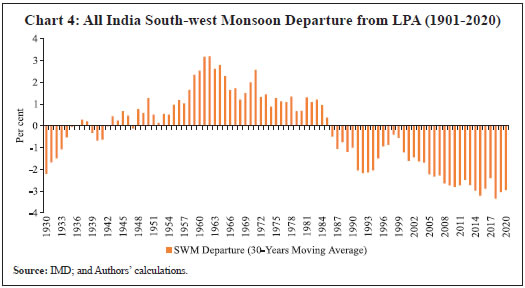 The frequency and intensity of floods and droughts are significantly associated with the spatial and temporal distribution of SWM in India. In addition, the occurrence of major floods and torrential rains has been reported largely since 2004, while unseasonal rainfall has been an increasing cause of worry since 2011 (Dilip and Kundu, 2020). In this paper, we study in detail the frequency of floods and droughts in the coastal states. We also make a spatial comparison of the regions within these states that are heavily affected by floods and droughts (Annex Table I). Data reveal that the eastern coastal states of West Bengal and Andhra Pradesh are more prone to the occurrence of floods and droughts. On the other hand, in the western coast, Karnataka and Maharashtra are the two states that have seen the highest frequency of floods and droughts during 1951-2020 (Chart 5). In the case of Karnataka, the interior regions of the state are more prone to droughts, while the northern interior region is more prone to floods as compared to the southern interior region. The Central and Vidarbha regions of Maharashtra are more prone to the occurrence of droughts, while both Marathwada and Vidarbha regions are prone to floods. | Table 2: Frequency and Intensity of Droughts in India (1901-2020) | | Period | Drought Years
(South-west Monsoon Departure) | Drought Frequency
(Severe Droughts) | | 1901-1930 | 1901
(-13) | 1904
(-12) | 1905
(-17) | 1911
(-15) | 1918
(-25) | 1920
(-17) | | | | 6 (3) | | 1931-1960 | 1941
(-13) | 1951
(-19) | | | | | | | | 2 (1) | | 1901-1960 | 8 drought years (3 severe drought years) | 8 (3) | | 1961-1990 | 1965
(-18) | 1966
(-13) | 1968
(-10) | 1972
(-24) | 1974
(-12) | 1979
(-19) | 1982
(-15) | 1986
(-13) | 1987
(-19) | 9 (4) | | 1990-2020 | 2002
(-19) | 2004
(-14) | 2009
(-22) | 2014
(-12) | 2015
(-14) | | | | | 5 (2) | | 1961-2020 | 13 drought years (5 severe drought years) | 14 (6) | Note: Here we have considered SWM departure below (-)10 per cent as drought years and below (-)15 per cent as severe drought years. While droughts are generally classified based on standardised precipitation index (SPI), different methods to obtain the SPI may significantly alter the classification of drought years (moderate to severe). Years in bold indicate severe drought years.
Source: IMD; Nandargi and Aman (2017); and Krishnan et al. (2020). | III.3.3 Rise in Sea Level The rise in sea level has a significant impact on the densely populated coastal areas and the low-lying islands around the globe. As noted by Krishnan et al. (2020), the Indian Ocean region is home to roughly 2.6 billion people (around 40 per cent of the global population) and is rich in marine ecosystem. Therefore, the rise in sea level poses a challenge to population, economy, coastal infrastructure and marine life. Further, some of the largest cities in India are located along India’s long coastline, which makes them extremely vulnerable to the impact of rising sea level with the risks including loss of land due to erosion, damage to coastal projects, infrastructure and power plants, salinisation of freshwater and increased vulnerability to flooding (Krishnan et al., 2020). Although data are not available for a comparable period in the Indian context, rising sea level can be witnessed in four major coastal locations viz., Mumbai, Kochi, Vishakhapatnam and Kolkata (Table 3). 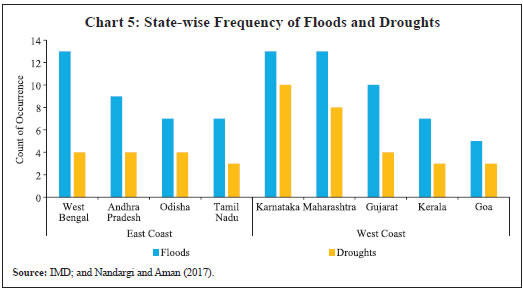
| Table 3: Trends in Sea Level Rise at Selected Tide-gauge Locations | | Station | Period | Trends in relative sea level rise (mm/year) | Net sea level rise trend (mm/year) | | Mumbai | 1878-1993 | 0.77 ± 0.08 | 1.08 | | Kochi | 1939-2007 | 1.45 ± 0.22 | 1.81 | | Visakhapatnam | 1937-2000 | 0.69 ± 0.28 | 0.93 | | Diamond Harbour (Kolkata) | 1948-2010 | 4.61 ± 0.37 | 4.96 | Note: Table shows sea level trends (relative to land surface) with glacial isostatic adjustment (GIA)-corrected net sea level trends.
Source: Unnikrishnan et al. (2015). | It can be seen that the maximum rise in sea level was witnessed in Diamond Harbour, Kolkata which is along the eastern coastline of India. This may be attributed to the higher frequency of cyclone occurrences along the eastern coastline. III.4 Impact of Climate Change on Agriculture Agriculture is one of the most important sectors of the Indian economy. The deviations in the pattern of SWM can adversely affect the agricultural sector and the macroeconomy. In the recent times, highest deficit in rainfall in terms of SWM departure from LPA was witnessed in 2014 and 2015. This period also witnessed late arrivals of SWM (Dilip and Kundu, 2020). Chart 6 shows the comparison of the growth rates in GSVA-Agriculture for coastal states with their neighbouring non-coastal states. It can be seen that lower than average rainfall is generally accompanied by lower growth in GSVA-Agriculture of coastal states. The negative growth rates are more prominent in the western coastal states than their eastern counterparts. Incidentally, during the considered time periods, the third strongest cyclone of the Arabian Sea, Nilofar, peaked in October 2014 causing damage along the western coastline. Like the coastal states, the non-coastal neighbouring states were also seen to be more affected in 2015-16. Section IV
Data and Description This section presents the data-related details for the empirical section of our paper. Our paper considers the nine coastal states of India and their eight non-coastal neighbours (Chart 7). The coastal states include the five states along the western coastline (Gujarat, Maharashtra, Goa, Karnataka and Kerala) and the four states along the eastern coastline (West Bengal, Odisha, Andhra Pradesh and Tamil Nadu). It may be reiterated that our paper purely focuses on the causal impact of the frequently occurring natural calamities (floods, droughts and cyclones) in the coastal states vis-à-vis their non-coastal neighbouring counterparts as these are some of the most densely populated states in India with large-scale economic activity and are adversely affected by these calamities almost every year. As seen in the earlier sections, floods and cyclones have amplified adverse impacts on infrastructure and livelihood and are responsible for a significant number of human casualties in India. Although flood and drought affect both coastal and non-coastal parts of the country, anecdotal evidences suggest that their intensities are more in the coastal states. Moreover, cyclones generally originate in either the Bay of Bengal or the Arabian Sea and, therefore, are more frequent in coastal states. The frequency of inland cyclones in India is minimal. The cyclone proneness of the different districts of India for the period from 1891 to 2008 reveals that districts along the eastern coastline are more prone to cyclones as the highest frequency of cyclone occurrences is witnessed in the districts of West Bengal and Odisha (Chart 8). 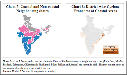 The sample period covered for the analysis is 2011-12 to 2019-20 and the natural calamities (extreme weather events based on frequency of occurrence) considered are floods, droughts and cyclones that occurred in the coastal statesduring this period (Annex Chart I).6 Although the sample period is short, the consideration of the data period is justified considering the continuously changing climatic patterns across the country. In comparison to the years prior to 2011-12, it is the past decade which has witnessed a considerable reduction in deaths due to extreme weather events (Chart 1a), a significant change in average rainfall pattern (Chart 2a), a drastic increase in maximum temperature (Chart 2b) and changes in SWM departure from LPA (Chart 4). Further, the consideration of this sample period eliminates the possible impact of structural changes in macroeconomic variables and introduction of new base years for some of them. The details of the intensity of the calamities during the period under consideration are provided in Annex Table II. In order to study the causal effects of the green swan events on macroeconomic and financial variables (including income, agricultural yields, tourism, inflation, fiscal parameter and cost of borrowings) of coastal states by controlling for the neighbouring landlocked states, state-wise data are obtained for all the considered 17 states. Annual growth rates are used in the case of most variables and the detailed description of variables along with their data sources is given in Annex Table III. The variables are categorised into five groups: (i) Output and per capita output; (ii) Agricultural yield; (iii) Inflation (headline and food inflation); (iv) Fiscal parameters (gross fiscal deficit, capital and revenue expenditures); and (v) Financial services [yields of State Development Loans (SDLs)], tourist visits, foreign direct investment (FDI) inflows, area insured under weather-based crop insurance). The data are sourced mainly from the National Statistical Office (NSO) under the Ministry of Statistics and Programme Implementation (MoSPI); Department of Agriculture, Cooperation and Farmers Welfare (DAC&FW) under the Ministry of Agriculture and Farmers Welfare (MoAFW); and the Reserve Bank of India (RBI)’s State Finance: A Study of Budgets. The select dependent variables aim to represent different aspects of the Indian macroeconomy. The causal impact of green swan events on macroeconomic variables like income, growth, inflation, tourism and agricultural yields is intuitional and straight-forward. In order to meet the targets of pollution curtailment as per the PA, the Government may introduce new environmental policies, including fiscal measures impacting both taxation and expenditure. Therefore, it would be interesting to analyse the impact of green swans on fiscal parameters. Further, the occurrence of green swan events may trigger negative sentiments among the investors and this could adversely affect the cost of borrowing and investment inflows. By considering SDL yields and FDI inflows, we explore the impact of green swans on market sentiments. In order to review the extent of implementation, utilisation and efficiency of measures taken by the Government to ameliorate the adverse effects of climate-related risks, the causal impact of green swan events on weather-based crop insurance, in terms of area insured is analysed. Section V
Empirical Findings V.1 Methodology Our objective in this paper is to study the causal effects of natural calamities on an array of macro variables that include GSDP, agricultural yield, fiscal variables, and a set of financial variables. In the absence of random draws, we use the D-i-D strategy to evaluate the causal effects of these calamities (random experiments), by splitting our sample into treatment and control groups. From geographical locations, we first identify the coastal states as these have been repetitively impacted by natural calamities in the recent years; this constitutes the treatment group for our study. Next, we select a set of neighbouring landlocked states that are: (i) less affected by the natural calamities; and (ii) similar in terms of production and household behaviour. These are the control set of states for our experiment. Though the treatment and control sets are not perfectly comparable, we try to achieve the best matching, in view of the common trend assumption in the D-i-D models. Then we compare the deviation in the common trend between the treatment (coastal) states and the control (neighbouring but landlocked) states before and after an experiment (the occurrence of a natural calamity in our case). The central assumption is that the unobserved differences between the treatment and control groups that are unrelated to natural calamity must be common over time, and therefore, will be cancelled out while differencing, and therebyaddress the omitted variables problem.7 V.1.1. Model Specification Our basic D-i-D-equation includes four variables: the dependentvariables (yit), a dummy for the treatment states (coastalD), another dummy for the natural experiments, which takes the value one for the calamity years, and zero otherwise (calyearD), and finally an interaction term, which is generated by multiplying these two dummies (D-i-D=coastalD*calyearD).8 This is a typical research design in a D-i-D model, where the coefficient of the interaction term captures the causal effect of the natural calamity. Thus, our basic regression model is as under: We use each of the state specific macro variables (an exhaustive list is reported in Annex Table III) as dependent variables in our model. Then in each of the regressions, the coefficients could be interpreted as follows: In equation 1, coefficient β1 captures systematic differences between our treatment group and control group, while β2 captures the changes in the treatment group vis-a-vis the control group during the calamity times,which is our natural experiment.9 Finally, and perhaps the most important one is the coefficient δ, which captures the difference between the changes in the coastal states compared to the non-coastal states during the natural calamity years. In our second model, we modify the interaction term (D-i-D) to include its lead and lag. This helps us to analyse the changes in the dependentvariables yit in the coastal states relative to their neighbouring states one year preceeding the natural calamity and one year succeeding the calamity. Ourmodified set of equation is as under: Where, there are three coefficients of δ that help us to compare calamity year with its immediate past and future.10 In our next research design, we replace the uniform coastal dummy(coastalD) by a set of dummies for each state, excluding one. Similarly, we create time dummies for each year, excluding one, for the sample group. This is in the spirit of a fixed effect panel data model, which helps us to control for each of the state specific and time specific effects. Finally, we introduce the D-i-D dummy for estimating the causal interferences. This is in spirit of the research design followed by Angrist and Pischke (2014) in their analysis of Minimum Legal Drinking Age (MLDA) regressions for US. The regression equation is as under:  While such a regression setup helps us to control for any state or time specific effects and relax the common trend assumption, there is a caveat. Such a regression would generally require a large number of observations to estimate all state and time dummies. In the MLDA case, there were 14 years of data for 51 states leading to 714 observations. However, in our case there are a total of 136 observations, and therefore, the estimated coefficients might have some small sample biases. Using weighted regression rather than ordinary least squares (OLS) generally increases the precision of the regression estimates. Considering the possibility of differences in error variance across states, we consider a cross-section weighted feasible generalised least squares (GLS) specification assuming the presence of cross-sectional heteroscedasticity. In such a specification, inverse of standard errors across groups are used as weights. Further, as state-year panel stacks observations on states over time, they often report serial autocorrelation over time within states or within the same period between states. In such a situation our hypothesis testing result may lead to misleading conclusions. To address this problem, we use clustered standard errors, which takes into account any sort of period dependence observed in the sample dataset. Based on these three equations, our empirical findings are discussed in the following sub-sections. V.1.2 Matching of Treatment and Counterfactual States Section IV presented the analysis for the coastal states and their non-coastal neighbouring counterparts. A district-wise matching would have been a better approach as against the state-wise matching based on the criterion if a state is coastal or not. However, the non-availability of data for most of the considered macroeconomic variables at the district level restricted us from performing the matching based on districts. While the states may be similar regarding some of the key macroeconomic parameters, the difference lies in the fact that the coastal states are directly and frequently impacted by the natural calamities such as cyclones as compared to their neighbouring non-coastal counterparts which are impacted only indirectly. The causal inference used in the empirical analysis is based on these characteristics of coastal states and their neighbouring inland states, thus conferring to the requirements ofD-i-D framework.11 In terms of key macroeconomic indicators like GSDP and per capita net state domestic product (NSDP), the coastal states share similarities with theirnon-coastal neighbouring counterparts.12 To achieve a state level matching, state-level correlations were computed spanning the entire sample period for these economic variables, which also reveal similarities with the neighbouring states (Annex Tables IV a and b). The pattern of crop production based on favourable farming conditions across the geographically neighbouring states also indicate certain similarities. For instance, Maharashtra, Madhya Pradesh, Rajasthan, Andhra Pradesh and Karnataka are some of the largest producers of pulses and maize in India, while West Bengal, Assam and Bihar are some of the key producers of jute and paddy. Gujarat, Maharashtra and Rajasthan are the key producers of oilseeds. Furthermore, the average headline inflation ranged between 5.3 per cent and 6.5 per cent for the coastal and non-coastal states during the period under consideration. The correlation matrices, based on the entire sample period, presented in Annex Tables V to VIII reveal that the matching of states (treatment group versus placebo group) may not be entirely full-proof as some of the neighbouring states do not share a significantly high correlation across allthe select macroeconomic parameters considered in our study.13 Therefore, all the select macroeconomic parameters and the coefficients may not be perfect as some of the neighbouring states do not share a significantly high correlation. To address this particular concern, we estimate Model-3 [equation(3)] wherein we replace the uniform coastal dummy (coastalD) by a set of dummies for each state (excluding one), and for each year (excluding one) for the sample group. This method, following Angrist and Pischke (2014), is a useful one because it allows for every state to have a different intercept term, which captures that all states are differently placed. As noted by Angrist and Pischke (2014) “... Samples that include many states and years allow us to relax the common trends assumption, that is, to introduce a degree of non-parallel evolution in outcomes between states in the absence of a treatment effect”. Further, there could be a possibility that the selected set of states might have a different time trend altogether and are not comparable under the D-i-D framework. To check for this possibility, following Rambachan and Roth (2019) and Bilinski and Hatfield (2018), we then assume that the pre-existing difference in trends persists, and to simply extrapolate this out we introduce a time trend t [index time from (1, ..., T)] and coastal state dummy interaction by augmenting Model-3. This coefficient, if found significant, assumes that the difference in trends would continue to hold. However, the coefficient associated with the time dummy for our sample turned out to be statistically insignificant. Though a typical regression coefficient test or propensity matching test of parallel trends may not be appropriate in the present set-up, we attempted to ensure that untreated units provide the appropriate counterfactual based on a reasonable set of logical assumptions, which include neighbouring state matching, incorporating state-specific dummies for different intercepts, and by incorporating a time trend assumption. V.2 Output and Per Capita Output A core concern in policymaking is identifying the signs of expansions and contractions in economic activity. In this section, we attempt to evaluate the impact of natural calamities on GSDP, which is our dependent variable for the regression equations. We take GSDP growth rates rather than levels because, in an emerging market like India, we generally witness growth cycles rather than business cycles (Bhadury et al., 2021). Considering the heterogeneity of Indian states in terms of their size and population density, we also consider per capita NSDP growth for the states as a dependent variable. The basic D-i-D regression results [equation (1)] and the interaction coefficient (D-i-D) that reports the causal impact of natural calamities on GSDP growth of the coastal states are reported in Table 4 (columns 1 and 2). The interaction term reports a negative and significant coefficient when GSDP growth is taken as the dependent variable (Column 1). We also observe a similar negative and significant coefficient of the D-i-D term when per capita NSDP is used as the dependent variable. | Table 4: Full Sample Results (Contd.) | | | Output and Per Capita Output | Agricultural Productivity | | GSDP | Per Cap. NSDP | GSVA Agri | Foodgrains Yield | Vegetables Yield | Fruits Yield | | (1) | (2) | (3) | (4) | (5) | (6) | | Coastal Dummy | 1.42***
(0.09) | 6.39***
(0.79) | -7.01***
(1.86) | 0.20*
(0.11) | 6.21***
(0.51) | 2.28***
(0.25) | | Calyear Dummy | 0.99
(1.09) | 5.52***
(0.25) | -9.91***
(0.82) | 0.02
(0.05) | 0.31***
(0.08) | 0.64**
(0.20) | | D-i-D | -1.24***
(0.29) | -5.62***
(0.84) | 6.96***
(2.00) | 0.11
(0.07) | -0.52***
(0.09) | -0.65**
(0.26) | | Constant | 6.01***
(1.08) | - | 10.28***
(0.38) | 1.86***
(0.04) | 13.29***
(0.18) | 12.72***
(0.28) | | N | 122 | 122 | 122 | 119 | 111 | 110 | | R2 | 0.04 | -0.19 | 0.21 | 0.20 | 0.83 | 0.13 | | F Statistic | 1.63 | - | 10.51 | 9.57 | 170.88 | 5.13 |
| Table 4: Full Sample Results (Concld.) | | | Fiscal Parameters | Tourism and Other Financial Services | | GFD | CAPEX | Revenue Exp. | Tourist Visits | Weather- Based Insurance | FDI Inflows | SDL Yields | | (7) | (8) | (9) | (10) | (11) | (12) | (13) | | Coastal Dummy | - | 1.06
(0.84) | -2.73*
(1.52) | 8.36***
(0.23) | -4.02
(4.33) | -6.58
(34.54) | -0.07***
(0.00) | | Calyear Dummy | - | 0.58
(1.03) | -2.12
(1.64) | 0.51
(1.51) | 42.24
(29.05) | -44.10
(41.20) | -0.02
(0.48) | | D-i-D | -0.02
(0.36) | 3.18**
(1.29) | 1.16
(1.82) | -2.61**
(0.85) | -14.14
(8.78) | 29.20
(51.86) | 0.11
(0.06) | | Constant | 3.15***
(0.33) | 3.41***
(0.95) | 15.50***
(1.40) | 5.97***
(0.60) | 5.39
(25.57) | 57.70
(34.54) | 8.12***
(0.46) | | N | 50 | 120 | 119 | 120 | 77 | 108 | 117 | | R2 | 0.00 | 0.09 | 0.06 | 0.20 | 0.11 | 0.03 | 0.003 | | F Statistic | 0.01 | 3.98 | 2.55 | 9.89 | 2.88 | 0.92 | 0.12 | | Note: ***Significant at the 1 per cent level; **Significant at the 5 per cent level; *Significant at the 10 per cent level. Heteroscedasticity consistent clustered standard errors in parentheses. | We also estimate equation (2), which includes the lead and lag of the interaction dummy in addition to the contemporaneous term. These results indicate that the coefficients associated with D-i-D(-1) (i.e., the lagged term) of GSDP growth and per capita NSDP growth are not statistically significant (Table 5). This is in line with our expectation as natural calamities are exogenous events. Further, as in the previous section, the contemporaneous coefficients were found to be statistically significant, supporting substantial damage in GSDP due to these calamities. Furthermore, the negative and significant coefficients after the natural calamity year indicate that the impact of natural calamities could be prolonged and may spill over to the subsequent years. It was indeed intriguing to find that some of these coefficients reported higher numbers as compared to the calamity years indicating long-lasting impact. | Table 5: Difference-in-Differences with lead-lag (Contd.) | | | Output and Per Capita Output | Agricultural Productivity | | GSDP | Per Cap. NSDP | GSVA Agri | Foodgrains Yield | Vegetables Yield | Fruits Yield | | (1) | (2) | (3) | (4) | (5) | (6) | | Coastal Dummy | 4.24***
(0.66) | 4.13***
(1.10) | -4.68**
(1.67) | 0.10
(0.15) | 4.59***
(0.56) | 2.32
(1.80) | | Calyear Dummy | -0.77*
(0.33) | -1.22**
(0.37) | -16.58***
(0.75) | -0.01
(0.07) | 0.12
(0.10) | 0.77
(0.84) | | D-i-D(-1) | -0.82
(0.51) | -0.41
(0.84) | -8.12***
(0.96) | 0.02
(0.02) | 0.13
(0.39) | 0.59*
(0.28) | | D-i-D | -1.79***
(0.31) | -1.15**
(0.44) | 8.51***
(1.18) | 0.17*
(0.10) | -0.14
(0.25) | -0.88
(0.88) | | D-i-D(+1) | -1.96***
(0.24) | -2.07***
(0.41) | 3.73***
(0.79) | 0.05
(0.04) | 1.21***
(0.23) | 0.23
(0.22) | | Constant | 7.72***
(0.00) | 6.44***
(0.00) | 15.58***
(0.00) | 1.89***
(0.04) | 13.50***
(0.00) | 12.47***
(1.20) | | N | 102 | 102 | 102 | 102 | 96 | 95 | | R2 | 0.13 | 0.19 | 0.38 | 0.21 | 0.78 | 0.17 | | F Statistic | 2.87 | 4.51 | 11.53 | 4.95 | 62.31 | 3.71 |
| Table 5: Difference-in-Differences with lead-lag (Concld.) | | | Fiscal Parameters | Tourism and Other Financial Services | | GFD | CAPEX | Revenue Exp. | Tourist Visits | Weather- Based Insurance | FDI Inflows | SDL Yields | | (7) | (8) | (9) | (10) | (11) | (12) | (13) | | Coastal Dummy | - | 2.18
(9.99) | -9.10***
(2.75) | 5.73**
(2.15) | 18.32
(39.50) | 8.69
(42.92) | -0.35***
(0.10) | | Calyear Dummy | - | -1.12*
(0.46) | -0.56
(2.47) | -3.05*
(1.40) | 130.71***
(29.71) | 37.97
(30.80) | 0.85***
(0.08) | | D-i-D(-1) | 0.37
(0.37) | 4.13
(5.40) | 1.87*
(0.95) | -0.27
(1.21) | -49.66***
(13.43) | 39.60
(21.46) | 0.18***
(0.04) | | D-i-D | -0.24
(0.33) | -2.11
(4.52) | 2.71
(2.80) | 0.98
(1.76) | -19.23
(34.28) | -55.12
(34.40) | 0.12
(0.10) | | D-i-D(+1) | 0.53
(0.33) | 3.85
(4.85) | 3.42***
(1.22) | -3.29**
(1.03) | 16.74
(15.92) | 17.70
(21.46) | 0.22***
(0.06) | | Constant | 2.74***
(0.69) | 5.07***
(0.00) | 15.19***
(2.06) | 11.53***
(0.00) | -73.68***
(27.28) | 7.28***
(0.00) | 7.43***
(0.07) | | N | 42 | 101 | 100 | 101 | 72 | 102 | 99 | | R2 | 0.06 | 0.17 | 0.14 | 0.08 | 0.63 | 0.03 | 0.40 | | F Statistic | 0.81 | 3.82 | 3.11 | 1.67 | 22.29 | 0.67 | 12.34 | | Note: ***Significant at the 1 per cent level; **Significant at the 5 per cent level; *Significant at the 10 per cent level. Heteroscedasticity consistent clustered standard errors in parentheses. | Further, we estimate equation (3), which includes dummies for each state and year, and thereby controls for state specific heterogeneities and other evolving macroeconomic changes over the years. When GSDP growth is used as the dependent variable, the D-i-D coefficient reports a negative and significant coefficient, which supports our earlier findings (Table 6). | Table 6: Difference-in-Differences with Cross-section (State) and Time Dummies (Contd.) | | | Output and Per Capita Output | Agricultural Productivity | | GSDP | Per Cap. NSDP | GSVA Agri | Foodgrains Yield | Vegetables Yield | Fruits Yield | | (1) | (2) | (3) | (4) | (5) | (6) | | D-i-D | -0.73*
(0.38) | -0.82
(0.90) | 4.57***
(1.41) | 0.22***
(0.03) | -0.71
(0.45) | -0.21
(0.68) | | Cross Section Dummy | Yes | Yes | Yes | Yes | Yes | Yes | | Time Dummy | Yes | Yes | Yes | Yes | Yes | Yes | | Constant | 7.60***
(0.15) | 6.34***
(0.36) | 0.29
(0.58) | 1.96***
(0.01) | 16.73***
(0.16) | 14.08***
(0.25) | | N | 122 | 122 | 122 | 119 | 111 | 110 | | R2 | 0.44 | 0.45 | 0.35 | 0.91 | 0.87 | 0.91 | | F Statistic | 3.14 | 3.26 | 2.16 | 41.50 | 26.64 | 42.16 |
| Table 6: Difference-in-Differences with Cross-section (State) and Time Dummies (Concld.) | | | Fiscal Parameters | Tourism and Other Financial Services | | GFD | CAPEX | Revenue Exp. | Tourist Visits | Weather- Based Insurance | FDI Inflows | SDL Yields | | (7) | (8) | (9) | (10) | (11) | (12) | (13) | | D-i-D | 0.01
(0.40) | 4.14**
(1.71) | 0.64
(2.62) | -2.02
(1.91) | 0.93
(12.39) | -0.39
(91.54) | 0.02
(0.06) | | Cross Section Dummy | Yes | Yes | Yes | Yes | Yes | Yes | Yes | | Time Dummy | Yes | Yes | Yes | Yes | Yes | Yes | Yes | | Constant | 3.38***
(0.38) | 5.24***
(0.64) | 12.34***
(1.14) | 11.40***
(0.83) | 34.39***
(5.31) | 57.90
(37.29) | 8.11***
(0.03) | | N | 50 | 120 | 119 | 120 | 77 | 108 | 117 | | R2 | 0.72 | 0.45 | 0.25 | 0.30 | 0.54 | 0.19 | 0.95 | | F Statistic | 15.43 | 3.18 | 1.32 | 1.72 | 3.09 | 0.84 | 66.08 | | Note: ***Significant at the 1 per cent level; **Significant at the 5 per cent level; *Significant at the 10 per cent level. Heteroscedasticity consistent clustered standard errors in parentheses. | Our empirical results indicate that natural calamities cause a decline in GSDP growth and per capita NSDP growth. Further, the results also suggest that such calamities could have a lingering impact on income growth and revival could take time, as indicated by the signs and higher magnitudes of the D-i-D(+1) coefficients in Table 5 (columns 1 and 2). This implies that the impact of calamity impacts on output growth could last at least more than a year and might signal lingering macroeconomic risks. Our findings are in line with Cavallo and Noy (2011). The study presented cross-country evidence and argued that natural disasters generally have a negative effect on economic growth. Turning to the EMEs and neighbouring countries of India, Karim (2018) for Bangladesh and Kurosaki (2015) for Pakistan documented adverse impact of natural disasters on income and growth. In the case of India, a recent study found both short-run and medium-run negative impact on economic growth (Sandhani et al., 2020). The study shows that for poorer districts, a rise in temperature by 1oC leads to around 4.7 per cent decline in the growth rate of district per capita income. V.3 Agricultural Productivity Although the share of agriculture in the national income has been declining over the years, it still accounts for large-scale rural employment generation. Disruptions in foodgrains and vegetables production can result in volatility in inflation. Considering its overall importance and its dependence on weather conditions, particularly rainfall, we analyse the impact of natural calamities on agricultural productivity in this section. Following the seminal paper by Fisher (1925), we use yields of foodgrains, vegetables and fruits for our selected set of states as the dependent variables, as yields help us to standardise production per hectare of land and then compare the impact between coastal and inland states. We estimate equation (1). The D-i-D coefficients for vegetables yield and fruits yield are reported in columns 5 and 6 of Table 4. These coefficients are negative and significant indicating that natural calamities cause a decline in vegetables yield and fruits yield, which is on expected lines. However, we did not find strong empirical evidence from equations (2) and (3), as most of these coefficients were found to be statistically insignificant. Turning to foodgrains yield, most of its coefficients are found to be positive, though mostly statistically insignificant. The D-i-D coefficient for foodgrains yield in equation (3) reported a small positive value (Table 6, column 4) and was statistically significant. Though contradictory, these results are in line with Albala-Bertrand (1993) that documented positive impact of natural disasters on agricultural output, and Loayza et al. (2012) which concluded that small disasters might, on an average, positively impact the macroeconomy. For India, natural disasters in the coastal states may not have a major impact on foodgrains production in their inland districts, and therefore, yield of foodgrains may not indicate a significant deterioration. Since foodgrains constitute a major portion of the gross value added (GVA) in the agricultural sector, we estimated all the three regressions using growth in agricultural GVA as the dependent variable and found empirical support of increase in agricultural GVA from the coastal states. While our results did not show any adverse impact of natural calamities on the yield of foodgrains, their impact on the quality of foodgrains is difficult to estimate using this framework. The results could also indicate the significant role of policy interventions by the Government towards developing climate-resilient production techniques, particularly with respect to foodgrains, such as introducing drought/flood/temperature tolerant varieties in paddy and pulses in these states; water-saving paddy cultivation methods, advancement of rabi planting dates in areas with heat stress; and community nurseries assolutions for delayed monsoon arrival (NICRA14, 2016). V.4 Tourism Tourism is an important segment of the Indian economy because of its horizontal and vertical linkages to several employment intensive ancillarysegments. It accounts for around 7 per cent of the national GDP15 and a significant percentage of GSDP of some of the coastal states (e.g., Goa and Kerala). Travel and tourism (T and T) is the largest segment of commercialised leisure, and as per the World Travel and Tourism Council, its contribution to the GDP and employment of the Asia-Pacific (APAC) region in 2019 stood at 9.9 per cent and 10.0 per cent, respectively. Expenditure in T and T (and leisure in general) is one of the important channels of transfer from upper-income households to lower-income workers. Considering its importance in overall services sector, some of the GDP nowcasting and forecasting models include activities in tourism sector as a coincident or lead indicator (Bhadury et al., 2021). In this section, we attempt to analyse the causal impact of natural calamities on this crucial industry by considering state-wise total tourist arrivals as the dependent variable in our D-i-D framework. In equation (1), which is our base model (Table 4, column 10), the interaction coefficient D-i-D is negative and significant, indicating that natural disasters cause a decline in tourist arrivals. In the same table, the coefficient of coastal dummy reports a positive and significant coefficient, indicating that tourist arrivals in the coastal states (the β1 coefficient) are more than that of non-coastal states. Empirical results from equation (2), on the other hand, indicate that such natural calamities may have a lasting impact on tourist arrivals, as the coefficient of lead D-i-D is also found to be negative and significant (Table 5). These results are in line with the findings reported in Bloesch and Gourio (2015) for US states and Dilip and Kundu (2020) for India, supporting the view that weather conditions impact economic activity particularly in sectors such as utilities, hospitality and retail segments. Tourism industry is perceived to have huge potential and is particularly an important source of income in some of the states. It has deep-rooted connections with the labour-intensive ancillary segments. Foreign tourist arrivals and air passengers had been secularly improving in India prior to the emergence of COVID-19 and the declaration of global lockdown particularly in 2020. The arrival of foreign tourists recorded an increasing trend during January 2003-March 2020 (Annex Chart IIa). The industry has also documented a seasonal pattern (Annex Chart IIb), which is a source of predictable income for many of the states. Our results indicate an adverse impact of natural disaster on this industry, which could also spill over in the immediate future years. V.5 Inflation To examine the impact of the natural calamities on inflation, we consider both headline inflation and food inflation for the select states. Favourable weather conditions are a prime requirement for maintaining robust agricultural output in any economy. In the case of India, the production and domestic availability of agricultural commodities are heavily dependent on conducive weather conditions. Weather-driven adverse supply shocks are a major cause of concern to the policymakers as they severely distort food prices. Since the food group constitutes a significant share (46 per cent) of the overall consumption basket in the all India consumer price index-combined (CPI-C), any upsurge in food prices not only pose significant upside risks for the headline inflation trajectory but may also feed into inflation expectations. Given this backdrop, we expect natural calamities in the coastal states to have an adverse effect on their food inflation vis-à-vis their non-coastal neighbours, implying that an occurrence of a natural calamity (cyclone; flood; drought) is expected to increase food inflation in the coastal states as compared to that in their non-coastal neighbouring counterparts. It is also expected that headline inflation, largely via the channel of food prices, would also increase in the coastal states owing to the occurrence of the natural calamity. V.5.1 Annual Inflation The impact of natural calamities on both headline and food inflation is presented in Table 7a. The basic D-i-D regressions with headline inflation and food inflation as the dependent variables in two separate models are presented in equation (1). The interaction coefficient (D-i-D) indicates the causal impact of the natural calamities on inflation, which is positive and statistically significant. The results suggest that the impact of natural hazards considered in the study is higher on food inflation as compared to headline inflation. The results in the generalised model, i.e., equation (3), has positive and significant (D-i-D) coefficients and thus, support results from equation (1), indicating that a sudden spike in inflation is caused by the natural calamities. The results corresponding to equation (2), which incorporates the lead and lag terms along with the contemporaneous term of the interaction dummy, seem to suggest that the natural calamities do not have a lasting and persistent impact on inflation, and interestingly available literature supports this result. Studies have found evidence that the impact of natural hazards on food inflation is generally positive and short-lived (Parker, 2018; Freeman et al., 2003; NGFS, 2020). However, Parker (2018) showed that the impact is heterogenous with respect to the type of the hazard and varies between advanced and developing economies. While storms may cause an immediate increase in food inflation, the impact could be reversed subsequently, resulting in no significant impact during the calamity year. Floods also have an immediate impact on food prices, especially in developing economies, and the impact lasts only in the period of flooding. Droughts, on the other hand, may cause headline inflation to rise significantly and the impact may persist for long. In the Indian context, it has been generally observed that the impact of a weather-induced supply shock (especially, floods/droughts) on food prices is largely restricted to perishable items (especially, vegetables and fruits) and the duration of the impact usually lasts for around 5-6 months (Dilip and Kundu, 2020). Pro-active supply management measures taken by the Government have a significant role in containing food price pressures. Our sample period is heavily skewed towards the incidence of floods and cyclones, which generally do not have a lasting impact on inflation. Therefore, in this section, unlike in the case of other macro-economic indicators (especially, GDP), equation (2) may not be an ideal/appropriate way of modelling the impact of the select natural calamities on inflation using annual data. | Table 7a: Inflation – Full Sample Results (Annual Data) | | Explanatory Variables | Equation (1) | Equation (2) | Equation (3) | | Headline Inflation | Food Inflation | Headline Inflation | Food Inflation | Headline Inflation | Food Inflation | | (1) | (2) | (3) | (4) | (5) | (6) | | Coastal Dummy | -0.84***
(0.17) | -0.44**
(0.18) | 2.01
(2.92) | 6.18
(6.08) | - | - | | Calyear Dummy | -2.63
(1.85) | -4.35
(3.10) | 0.55
(1.03) | 0.52
(1.62) | - | - | | D-i-D (-1) | - | - | -2.10
(2.35) | -4.08
(4.34) | - | - | | D-i-D | 0.96***
(0.24) | 1.11***
(0.31) | -0.37
(1.18) | -1.28
(2.26) | 0.65***
(0.19) | 1.25***
(0.34) | | D-i-D (+1) | - | - | -0.34
(0.10) | -2.27
(2.46) | - | - | | Constant | 7.98***
(1.65) | 7.97***
(2.38) | 5.01***
(0.00) | 4.66***
(0.00) | 5.67***
(0.08) | 4.43***
(0.14) | | Cross-section Dummy | - | - | - | - | Yes | Yes | | Time Dummy | - | - | - | - | Yes | Yes | | N | 136 | 136 | 102 | 102 | 136 | 136 | | R2 | 0.13 | 0.11 | 0.11 | 0.11 | 0.84 | 0.91 | | F Statistic | 6.63 | 5.49 | 2.44 | 2.39 | 24.15 | 47.20 | | Note: ***Significant at the 1 per cent level; **Significant at the 5 per cent level; *Significant at the 10 per cent level. Heteroscedasticity consistent clustered standard errors in parentheses. | V.5.2 Monthly Inflation Due to the availability of state-level monthly inflation data (January 2012-March 2021), we repeat the above analysis using month-wise headline inflation and food inflation. Here, we replace the calamity year dummy in equations (1), (2) and (3) with the calamity month dummy, where the dummy variable takes the value 1 for the calamity month and the value 0 otherwise. Table 7b presents the regression results. | Table 7b: Inflation – Full Sample Results (Monthly Data) | | Explanatory Variables | Equation (1) | Equation (2) | Equation (3) | | Headline Inflation | Food Inflation | Headline Inflation | Food Inflation | Headline Inflation | Food Inflation | | (1) | (2) | (3) | (4) | (5) | (6) | | Coastal Dummy | -0.09
(0.07) | 0.38***
(0.13) | -0.06
(0.11) | 0.28
(0.22) | - | - | | Calmonth Dummy | -0.45
(0.86) | 0.34
(1.46) | -0.46
(0.86) | 0.32
(1.37) | - | - | | D-i-D (-1) | - | - | -0.13
(0.61) | 0.61
(1.19) | - | - | | D-i-D | 0.37**
(0.16) | 0.45*
(0.28) | 0.49*
(0.28) | 0.41
(0.45) | 0.37**
(0.35) | 0.46*
(0.28) | | D-i-D (+1) | - | - | -0.38
(0.80) | -0.34
(1.41) | - | - | | Constant | 6.06***
(0.27) | 5.84***
(0.43) | 6.07***
(0.27) | 5.93***
(0.42) | 5.97***
(0.01) | 6.08***
(0.02) | | Cross-section Dummy | - | - | - | - | Yes | Yes | | Time Dummy | - | - | - | - | Yes | Yes | | N | 1853 | 1788 | 1819 | 1768 | 1853 | 1788 | | R2 | 0.001 | 0.004 | 0.003 | 0.004 | 0.76 | 0.77 | | F Statistic | 0.74 | 2.24 | 0.92 | 1.57 | 42.59 | 46.82 | | Note: **Significant at the 1 per cent level; **Significant at the 5 per cent level; *Significant at the 10 per cent level. Heteroscedasticity consistent clustered standard errors in parentheses. | We find that the results are broadly similar to that of the annual data, however, the coefficients are relatively lower in magnitude (in annual data there could be multiple calamities spread across months vis-à-vis monthly data where the impact largely captures the average impact per calamity ina month).16 Interestingly, the coefficients associated with food inflation are higher in magnitude as compared to those of headline inflation. The adverse impact of natural calamities on food inflation is also substantiated by Annex Chart III. It shows that the calamity frequency is especially higher during the monsoon season (June-September), which also coincides with the major crop sowing season (kharif) in India. To summarise, our empirical results with respect to inflation indicate that natural calamities have a positive impact on both food inflation and headline inflation with the impact being short-lived and generally restricted to the period of the calamity. Although transitory, the adverse impact on prices generally pose challenges for short-term inflation forecasting that involves nowcasting and near-term forecasting. Moreover, since short-term forecasting models are the satellite models feeding into the medium-term forecasting framework, forecast accuracy in the former becomes crucial from policy perspective. So far, climate-related risks have not been a major challenge for medium-term price stability in India under the flexible inflation targeting (FIT) framework. However, with the rising frequency and intensity of natural calamities, it is important that advanced climate-resilient horticulture techniques are adopted faster and effective supply management measures with a focus on processing, warehousing and storage facilities for the perishables (vegetables and fruits) are developed in order to reduce crop damages (so far, climate-resilient production methods and supply management measures have been mainly targeted towards maintaining the supply of foodgrains in India). Moreover, as India develops further, the demand for vegetables and fruits is expected to pick up. The growing penetration of organised retail chains would also support the demand for these perishable food items. Thus, climate-related risks, which adversely affect their supply and in turn impact inflation, cannot be ignored. V.6 Fiscal Parameters State plays an important role when natural disasters affect life and livelihood as it is involved in safety and reconstruction work. In order to analyse the same, we primarily concentrate on changes in state’s expenditure pattern owing to natural disasters. Our base model [equation (1)] indicates a statistically insignificant revenue expenditure growth coefficient for the interaction dummy (Table 4,column 9)17. However, the D-i-D coefficient for capital expenditure (CAPEX) reported a positive and significant coefficient (Table 4, column 8). When we controlled for state and time-specific effects in equation (3), the D-i-D coefficient indicated a CAPEX growth during the natural calamity years (while revenue expenditure growth was found to be statistically insignificant), thus confirming the empirical findings of equation (1). This apparently conflicting empirical findings could be due to the fact that most of the rebuilding expenditures are generally classified as capital expenditure. Turning to the gross fiscal deficit (GFD) of the states, our results were not statistically significant across regression specifications. In India, generally, state governments play a predominant role in rescue, relief and rehabilitation measures following a natural disaster, while centre has been playing a supporting role in terms of relief aids (Annex Chart IV). As the recurrence of such disasters is increasing over recent years, it is perhaps time to make adequate room in state budgets, at least in the disaster-prone states. This has also been advocated by Balasubramanian (2019) for India and Nakatani (2021) for disaster-prone small countries (e.g., Papua New Guinea). Calamity risk budgeting and stress tests in the budgets of coastal states, especially in the states that experience natural calamities from medium to high intensity, may help mitigate the risks of these green swan events. V.7 Other Financial Services V.7.1 Cost of Borrowing - SDL Yields SDLs in India refer to sovereign securities issued by various Indian states to raise funds. These are generally issued for meeting the state budget shortfalls and yields of these securities are market-determined set by way of consent granted by the Centre under Article 293(4) of the Constitution of India. Each state can borrow through SDL up to a set (yearly) limit, and SDLs are eligible for the RBI’s repo and for meeting Statutory Liquidity Ratio (SLR) requirements. They are also eligible for assets as level 1 high-quality liquid assets (HQLA) for liquidity coverage ratio (LCR) maintenance in India, given that states are fiscal sovereigns driving power through the Constitution to raise resources. The cut-off yields of these securities are determined through the RBI’s dedicated electronic auction platform (e-Kuber), and secondary market transactions are on Negotiated Dealing and Order Matching System (NDS-OM) that is in line with other dated government securities. In theory, given the marketable nature of such securities, yield is likely to represent the financial health of the issuing state. Using SDL yields as a proxy, we therefore, attempt to evaluate whether a natural disaster could significantly affect borrowing costs or cost of funds. To analyse the same, we follow the D-i-D research design, as highlighted in section V.1, and evaluate the sign and significance of the interaction term or the D-i-D coefficients. Our regression results indicate that the D-i-D coefficients, though positive, are not statistically significant. These results are uniform across all the three equations (Tables 4, 5 and 6, column 13) indicating that natural disasters do not cause an increase in cost of funds (or SDL yields). The coastal dummy coefficient in equation (1) has a marginally (7 basis points) negative coefficient, which could be due to the fact that some of the financially strong states are in the coastal areas. This result of insignificant D-i-D coefficient is consistent with literature in the Indian context. Bose et al., (2011) and Saggar et al., (2017) found empirical evidence that suggest no observable relationship between borrowing spreads of SDLs and states’ fiscal health, and states could mobilise funds at similar or near similar yields for the similar securities (RBI, 2019). In India, as a market development measure, an Automatic Debit Mechanism (ADM) was introduced for state governments to increase the confidence of investors (RBI, 2020); wherein RBI has the power to repay SDLs. Therefore, SDLs are generally considered risk-free by market participants irrespective of the issuing states and are assigned a zero-risk weight in capital to risk-weighted assets (CRAR) calculations of banks. This may explain our findings regarding the insignificant coefficients of the cost of borrowing caused by these natural calamities. It could also be the case that so far market participants have assigned a limited impact of climate change risks on key macro outcomes of states and therefore, do not expect a higher risk premium on SDLs following a major climate event. V.7.2 Weather Based Insurance and FDI Inflows In India, restructured weather-based crop insurance scheme has been published by the DAC&FW, which cover major food crops (cereals, millets and pulses) and oilseeds, commercial / horticultural crops. All farmers, including sharecroppers and tenant farmers, growing the notified crops in the notified areas are eligible for coverage and the state-wise data for the same are available for some of our sample states. Based on the available data, we estimated the D-i-D coefficients for weather-based crop insurance. However, these coefficients were mostly statistically insignificant (Tables 4 to 6, column 11). This could be because of expanding coverage of such insurance schemes and the relatively lower coverage of farmers witnessed in recent years (Annex Chart V). We also have state-wise data on FDIs, which help to test the causal impact of natural calamities on FDI destinations. However, our regression coefficients were largely found to be statistically insignificant (Tables 4, 5 and 6; column 12). FDIs are generally long-term investments that are undertaken after a large number of field-studies and feasibility analyses. Therefore, it is possible that these projects closely consider the possibility of occurrence of such green swan events before investing and are often located in the inland districts. Therefore, natural calamities may not have significantly impacted the capital inflows. V.8 Natural Calamities in East Coast vis-à-vis West Coast India is a large country and the states on the eastern coast differ considerably from those in the western coast in terms of income, production, consumption and other behavioural patterns. Data presented in section III of our paper show that the eastern coastal states have seen a higher incidence of cyclones and floods than their western counterparts historically. However, the section also revealed some facts indicating that these green swan events have increased in the recent years on the western coast. Therefore, considering that the Arabian Sea has emerged as a major source of severe cyclones with their intensity aggravating over time, we analyse the devastation caused by these green swan events in the eastern coastal states vis-à-vis their western counterparts in this section. At the sub-sample level (eastern coastal states versus western coastal states), our empirical analysis indicates that natural calamities have a statistically significant negative impact on the GSDP growth of western coastal states, while for the eastern coastal states the impact is rather muted (Tables 8 a and b, Column 1). Turning to fiscal side, CAPEX shows a large positive coefficient for the western coastal states, which may indicate extensive rebuilding expenditure incurred by these state governments during/after these green swan events (Tables 8 a and b, Column 4). | Table 8a: Sub-Sample Results – Eastern Coastal States | | | Output and Per Capita Output | Fiscal Parameters | Tourism and Other Financial Services | | GSDP | Per Cap. NSDP | GFD | CAPEX | Revenue Exp. | Tourist Visits | Weather- Based Insurance | FDI Inflows | SDL Yields | | (1) | (2) | (3) | (4) | (5) | (6) | (7) | (8) | (9) | | Coastal Dummy | -0.85*
(0.47) | -0.36
(0.54) | 0.49***
(0.00) | -0.83
(0.68) | -0.34
(1.04) | 3.36
(3.38) | -0.09
(13.02) | 25.78
(29.45) | -0.04
(0.12) | | Calyear Dummy | -0.09
(0.35) | 0.03
(0.42) | 0.15
(0.12) | -0.37
(0.36) | -0.80
(0.81) | 1.23
(1.49) | 13.74
(13.83) | -25.82
(26.18) | -0.09
(0.08) | | D-i-D | 1.17**
(0.55) | 0.63
(0.63) | 0.49*
(0.22) | 0.69
(0.57) | -0.80
(1.17) | -1.80
(3.31) | -29.06*
(16.34) | -6.51
(43.71) | 0.04
(0.12) | | Constant | 7.14***
(0.33) | 5.93***
(0.41) | 2.65***
(0.00) | 4.56***
(0.36) | 13.21***
(0.84) | 8.34***
(1.39) | 23.57*
(11.77) | 44.91***
(15.40) | 8.17***
(0.05) | | N | 122 | 122 | 38 | 120 | 119 | 120 | 77 | 108 | 117 | | R2 | 0.23 | 0.01 | 0.19 | 0.01 | 0.03 | 0.02 | 0.06 | 0.03 | 0.01 | | F Statistic | 1.02 | 0.22 | 2.59 | 0.21 | 1.07 | 0.68 | 1.64 | 1.10 | 0.24 |
| Table 8b: Sub-Sample Results – Western Coastal States | | | Output and Per Capita Output | Fiscal Parameters | Tourism and Other Financial Services | | GSDP | Per Cap. NSDP | GFD | CAPEX | Revenue Exp. | Tourist Visits | Weather- Based Insurance | FDI Inflows | SDL Yields | | (1) | (2) | (3) | (4) | (5) | (6) | (7) | (8) | (9) | | Coastal Dummy | 1.47**
(0.70) | 1.58***
(0.57) | -1.55***
(0.37) | 4.72
(3.19) | -2.01*
(1.04) | 3.64
(2.45) | -10.40
(10.50) | 5.93
(8.80) | 0.05
(0.09) | | Calyear Dummy | 0.19
(0.34) | 0.43
(0.40) | 0.25
(0.46) | 1.21***
(0.37) | -2.06*
(1.07) | -2.83**
(1.31) | 22.53*
(11.12) | 14.71
(17.17) | -0.23***
(0.05) | | D-i-D | -1.01*
(0.54) | -0.94
(0.56) | 0.05
(0.40) | 5.89**
(2.80) | 2.75*
(1.41) | 1.71
(2.54) | 5.80
(13.97) | -27.70
(24.96) | -0.04
(0.10) | | Constant | 6.74
(0.27) | 5.30***
(0.37) | 4.19***
(0.41) | 3.17***
(0.36) | 13.78***
(0.71) | 9.58***
(1.05) | 19.74**
(7.77) | 33.28***
(6.97) | 8.23***
(0.06) | | N | 122 | 122 | 50 | 120 | 119 | 120 | 77 | 108 | 117 | | R2 | 0.06 | 0.07 | 0.37 | 0.24 | 0.04 | 0.14 | 0.08 | 0.01 | 0.05 | | F Statistic | 2.49 | 3.01 | 8.91 | 12.54 | 1.80 | 6.50 | 1.99 | 0.22 | 2.15 | | Note: ***Significant at the 1 per cent level; **Significant at the 5 per cent level; *Significant at the 10 per cent level. Heteroscedasticity consistent clustered standard errors in parentheses. | Next, we evaluate the impact of calamities on inflation of the western and eastern coastal states separately as the overall impact would be a result of how food inflation is impacted in the two treatment groups. The results are presented in Tables 9 a, b and c. The results corresponding to equations (1) and (3) are broadly similar and indicate that western coastal states experience a larger impact of the natural calamities on their inflation as compared to their eastern counterparts. In the case of eastern coastal states, the impact is restricted only to food inflation. One of the possible reasons could be differences in the production baskets of eastern coastal states vis-à-vis western coastal states. Literature has showed that natural calamities cause larger damage to the production and supply of perishable food items, particularly vegetables and fruits, and thus, pose a higher upside risk on their prices. The coastal states of India are some of the major producers of the primary vegetables (potato, tomato and onion) in the country. While the western coastal states of Maharashtra and Karnataka largely cater to onions and tomatoes, the eastern coastal states of West Bengal and Odisha are the major producers of potatoes and Andhra Pradesh is a key tomato supplier. India’s experience with floods/extreme rainfall events suggests a greater impact on the prices of onions and tomatoes as compared to that of potatoes since potatoes are relatively less perishable in nature as well as have a better supply management infrastructure with respect to availability of go-downs and cold storages. Further, the western coastal states are also some of the key producers of fruits like oranges and grapes, the production of which is also impacted by the natural calamities. The blossoming season of Nagpur orange generally overlaps the months when the frequency of natural calamities is high. Another reason could be that with repeated incidence of cyclones and floods, the eastern coastal states may have initiated and developed better crop management practices and climate-resilient horticulture techniques as compared to the west coast of India. | Table 9a: Inflation – Sub-Sample Results [Equation (1)] | | Explanatory Variables | Eastern Coastal States (Annual) | Eastern Coastal States (Monthly) | Western Coastal States (Annual) | Western Coastal States (Monthly) | | Headline Inflation | Food Inflation | Headline Inflation | Food Inflation | Headline Inflation | Food Inflation | Headline Inflation | Food Inflation | | (1) | (2) | (3) | (4) | (5) | (6) | (7) | (8) | | Coastal Dummy | 0.24
(0.36) | 0.08
(0.49) | 0.28*
(0.15) | 0.29**
(0.12) | -0.77***
(0.28) | -0.08
(0.40) | -0.32***
(0.09) | 0.10
(0.16) | | Calyear/Calmonth Dummy | -0.18
(0.54) | -0.79*
(0.40) | 0.35**
(0.15) | 1.59
(1.52) | -3.60***
(0.27) | -7.14***
(0.44) | -2.37***
(0.45) | -2.74***
(0.81) | | D-i-D | -0.18
(0.51) | 0.27
(0.88) | 0.22
(0.20) | 0.66*
(0.39) | 0.99*
(0.52) | 0.52
(0.71) | 1.01***
(0.22) | 1.10**
(0.48) | | Constant | 6.03***
(0.21) | 5.35***
(0.24) | 5.90***
(0.11) | 5.93***
(0.40) | 7.84***
(0.19) | 8.42***
(0.27) | 6.23***
(0.27) | 6.23***
(0.45) | | N | 136 | 136 | 1853 | 1788 | 136 | 136 | 1853 | 1788 | | R2 | 0.002 | 0.01 | 0.002 | 0.01 | 0.41 | 0.48 | 0.03 | 0.02 | | F Statistic | 0.10 | 0.24 | 1.76 | 5.39 | 30.25 | 41.02 | 20.81 | 10.11 |
| Table 9b: Inflation – Sub-Sample Results [Equation (3)] | | Explanatory Variables | Eastern Coastal States (Annual) | Eastern Coastal States (Monthly) | Western Coastal States (Annual) | Western Coastal States (Monthly) | | Headline Inflation | Food Inflation | Headline Inflation | Food Inflation | Headline Inflation | Food Inflation | Headline Inflation | Food Inflation | | (1) | (2) | (3) | (4) | (5) | (6) | (7) | (8) | | D-i-D | -0.04
(0.33) | 0.29
(0.24) | 0.26
(0.24) | 0.62*
(0.37) | 0.86**
(0.36) | 0.84
(0.60) | 1.09***
(0.28) | 1.18***
(0.47) | | Cross-section Dummy | Yes | Yes | Yes | Yes | Yes | Yes | Yes | Yes | | Time Dummy | Yes | Yes | Yes | Yes | Yes | Yes | Yes | Yes | | Constant | 5.94***
(0.05) | 4.88***
(0.04) | 5.99***
(0.00) | 6.10***
(0.01) | 5.81***
(0.05) | 4.80***
(0.09) | 5.98***
(0.01) | 6.09***
(0.01) | | N | 136 | 136 | 1853 | 1788 | 136 | 136 | 1853 | 1788 | | R2 | 0.84 | 0.91 | 0.75 | 0.77 | 0.84 | 0.91 | 0.76 | 0.77 | | F Statistic | 23.66 | 45.69 | 42.52 | 46.80 | 24.62 | 46.39 | 42.90 | 46.95 | | Note: ***Significant at the 1 per cent level; **Significant at the 5 per cent level; *Significant at the 10 per cent level. Heteroscedasticity consistent clustered standard errors in parentheses. |
| Table 9c: Inflation – Sub-Sample Results [Equation (2)] | | Explanatory Variables | Eastern Coastal States (Annual) | Eastern Coastal States (Monthly) | | Headline Inflation | Food Inflation | Headline Inflation | Food Inflation | | (1) | (2) | (3) | (4) | | Coastal Dummy | 0.20
(0.15) | 0.03
(0.24) | -0.26***
(0.10) | 0.19
(0.18) | | Calmonth Dummy | 0.35
(0.93) | 1.54
(1.57) | -2.38***
(0.45) | -2.81***
(0.81) | | D-i-D (-1) | 0.87
(0.96) | 2.82
(1.84) | -0.64
(0.46) | -0.42
(1.32) | | D-i-D | 0.29
(0.36) | 0.92**
(0.45) | 1.77***
(0.56) | 2.13*
(1.12) | | D-i-D (+1) | 0.02
(1.21) | 1.02
(1.94) | -1.32***
(0.44) | -2.18*
(1.29) | | Constant | 5.91***
(0.24) | 5.99***
(0.42) | 6.24***
(0.28) | 6.30***
(0.45) | | N | 1819 | 1768 | 1819 | 1768 | | R2 | 0.004 | 0.01 | 0.04 | 0.02 | | F Statistic | 1.46 | 4.88 | 14.73 | 7.87 | | Note: ***Significant at the 1 per cent level; **Significant at the 5 per cent level; *Significant at the 10 per cent level. Heteroscedasticity consistent clustered standard errors in parentheses. | We also consider looking at equation (2) comprising lead and lag interaction dummies along with the contemporaneous one, but we restrict our analysis only to monthly data. Table 9c presents the results. The results are largely in line with what we have obtained for equations (1) and (3), although the contemporaneous interaction dummy shows a higher coefficient for the west coast equations. Further, the coefficient associated with D-i-D(+1) turns out to be negative and significant, indicating that the impact of the calamity could be restricted only to the calamity month for the western coastal states. Our findings are broadly in line with the existing literature (Parker, 2018; Freeman et al., 2003; NGFS, 2020; Dilip and Kundu, 2020; Andersson et al., 2020). To sum up, our empirical results indicate that the impact of the natural calamities is higher on the western coastal states of India as compared to their eastern counterparts. Historically, since the eastern coastal states have seen a higher incidence of natural calamities (especially cyclones and floods), it seems that they have developed better adaptation mechanisms as compared with the western coastal states. Limited data available on projects related to natural disaster management measures show that the construction of multi-purpose cyclone shelters (MPCS) and underground cabling in the western coastal states are lagging behind their eastern counterparts in terms of project execution (Annex Charts VI a and b). Section VI
Green Swans and Public Policies in India Minimising the frequency, intensity and macroeconomic impact of green swan events demand well-designed and internationally coordinated policies. In this section, we try to present a brief note on the policy actions in this regard that have already been initiated in India so far. Through the creation of the National Disaster Management Authority (NDMA) in 2005, the Government of India (GoI) initiated a change in the approach to disaster management in the country, from a relief-centric approach to a more holistic and an integrated approach, that includes processes involving prevention, mitigation, preparedness, response, relief, reconstruction and rehabilitation. Further, the National Action Plan on Climate Change (NAPCC) was formulated in 2008 as a consolidated policy instrument with a focus on a broader set of measures towards adaptation and mitigation of climate change impact, natural resource conservation and promoting energy efficiency. Importantly, the Climate Change Finance Unit (CCFU) was formed in 2011 under the Ministry of Finance to serve as the nodal agency on matters related to ‘climate change financing’ in India. One of the major functions of this unit is to provide inputs towards the designing, operationalisation and working of the green climate fund in India. Access to green finance, which includes investments seeking to support the accomplishment of environmental objectives, would be a key driver that would tackle India’s fight against climate change. The CCFU is expected to function as a coordinating agency for the various institutions responsible for green finance in India. VI.1 Central Bank Initiatives RBI has been playing an instrumental role in steering green finance initiatives in India. As part of its green finance drive, the small renewable energy sector has been included under the Priority Sector Lending (PSL) scheme in 2015. Firms in the renewable energy sector are eligible for loans upto INR 30 crore and households are eligible for loans upto INR 10 lakh under this scheme for investing in renewable sources of energy. Moreover, through its various reports, publications and other communication platforms, RBI is actively sensitising the public, investors and banks towards the need, opportunities, and challenges of green finance in India. RBI has joined the Network for Greening the Financial System (NGFS) and interactions in the group are expected to bring significant learning effects for India and other participating countries. It can benefit from the membership by learning and contributing to the global efforts in green finance. The NGFS, launched in December 2017, is a group of 95 central banks and supervisors and 15 observers as of June 30, 2019. It is a voluntary platform where the members are committed to sharing best practices, contributing to the development of climate-related risk management in the financial sector and mobilising mainstream finance to support the transition to a sustainable economy. In its first comprehensive report published in April 2019, NGFS laid out six recommendations for central banks, supervisors, policymakers and financial institutions to enhance their role in the greening of the financial system and managing environment and climate-related risks, particularly the impact of physical and transition risks on business and society at large (NGFS, 2019). In the second report of NGFS, emphasis is given to a new set of climate scenarios by including countries’ commitments to reach net-zero emissions, and the setup of an online NGFS scenarios website providing access to all NGFS publications and data (NGFS, 2021). Some of the important initiatives taken by the central banks globally include: the European Central Bank’s (ECB’s) inclusion of global warming as a key part of its strategy review; Bank of England’s mandate to make its monetary policy greener; and People’s Bank of China’s inclusion of climate-related risks into the annual stress test of the banks in the country. The Dutch National Bank conducted an energy transition risk stress test to examine the vulnerabilities of financial institutions to a net-zero carbon future. Banque de France announced a comprehensive climate stress test for banks and insurance companies to assess their exposure to both physical and transition risks. With an increase in frequency and severity of green swan events, there is a likelihood for increase in default rates of loan portfolios. RBI may also consider recommending internal stress tests to the regulated entities to measure their financial exposures. Some of the other important measures that the central banks globally may examine to mitigate climate-related risks include strengthening their analytical models by incorporating climate-related indicators and factors, bridging data gaps related to various environmental aspects of finance and providing additional/subsidised liquidity support to banks investing in environmentally friendly products/green projects (Krogstrup and Oman, 2019). VI.2 Fiscal Initiatives There have been several fiscal measures and financial incentives at work in India with an aim to minimise climate-related risks and use of renewable sources of energy. For instance, the GoI offers 30 per cent of the installation cost of the rooftop solar panels as subsidy to the institutional, residential and social sectors in the non-special category states18. In someof the special category states19, the subsidy is up to 70 per cent of the installation cost. Further, the excess power can be sold at a tariff set by the government. Moreover, the GoI has launched two phases of Faster Adoption and Manufacturing of Hybrid and Electric Vehicles (FAME) scheme in 2015 and 2019 to enhance the flow of credit, reduce the upfront purchase price of all vehicles and develop the necessary infrastructure (such as charging stations) to encourage green vehicle production and sales in India (NITI Aayog, 2019). In order to counter the high upfront cost of such vehicles, the State Bank of India has introduced ‘green car loans’ for electric vehicles (EVs) with concessional processing fee and interest rates as compared to the existing car loans (Jain, 2020). The Union Budget 2022-23 took major initiatives to support green economy and green finance in India, which over time can help mitigate climate risks, including transition risks. An allocation has been made for INR 195 billion to boost manufacturing of solar modules under the Production Linked Incentive (PLI) scheme. Other initiatives include introduction of battery swapping policy for EVs, setting up of more EV charging stations and launch of sovereign green bonds to step up funding of green infrastructure. In times to come, India can explore the feasibility of introduction of carbon taxation as it can help firms and households to reduce emissions. The implementation of a carbon tax may result in producers investing in less carbon-intensive technologies. In the Indian context, as recommended by Patra et al. (2021), the focus should shift towards climate change through carbon pricing, once the ongoing health crisis ends. This may necessitate the incorporation of transition risks in the macroeconomic forecasting models. VI.3 Market Regulators20 One of the major strategic moves since 2015 involves the implementation of the sustainability disclosure requirements. The Securities and Exchange Board of India (SEBI) has made it mandatory for the top 100 listed companies in the Bombay Stock Exchange (BSE) and the National Stock Exchange (NSE) to publish their annual business responsibility reports. Subsequently, with effect from 2022-23, filing of Business Responsibility and Sustainability Report (BRSR) shall be mandatory for the top 1000 listed companies. In addition, the Ministry of Corporate Affairs imposed compulsory reporting of the progress on Corporate Social Responsibilities (CSR) under the CompaniesAct, 2013.21 In addition, with regard to the green financial institutions, Indian Renewable Energy Development Agency (IREDA), a government-backed agency for promoting clean energy investments, announced its plans to become India’s first Green Bank in May 2016. Further, the India Infrastructure Finance Corporation Limited (IIFCL) launched ‘credit enhancement scheme’ in 2012 termed for funding viable infrastructure projects with bond tenors above five years (Jain, 2020). SEBI, in 2015, also initiated a consultation process for disclosure requirements for issuance and listing of Green Bonds in India. The disclosure requirements were based on green bond principles that include the use and management of the proceeds; project evaluation and selection; project monitoring and progress report. Finally, given the large size of the domestic market and a smaller penetration of green instruments so far in India, there remain vast opportunities to be tapped. In this context, the need of the hour is (i) increased coordination between investment and environmental policies; and (ii) an implementable policy framework for both central and state governments in addressing the existing frictions. In this vein, RBI is actively pursuing some of the policy measures such as deepening of corporate bond market, and removing information asymmetry between investors and recipients which can go a long way in developing the green finance market infrastructure. Further, a developed commodity derivatives market can also help mitigate risks by enabling continuous price discovery and providing a strategy for hedging price risk during episodes of uncertainty. Section VII
Conclusion Climate change poses a major threat to the optimal functioning of an economy. Climate-related disasters, generally referred to as green swan events due to their unpredictable and cataclysmic character, pose significant physical and transition risks to the overall macroeconomic and financial outcomes. Our paper is unique in its construct and research design as it considers the Indian coastal states that are frequently impacted by some of the extreme weather events, particularly cyclones, unseasonal rains and floods in addition to droughts to study the effects of these natural calamities on their macroeconomic outcomes as compared with their non-coastal neighbouring counterparts. Using a difference-in-difference panel data based econometric approach, the paper analyses the causal impact of the green swan events on macroeconomic indicators such as output growth, agricultural yields, inflation, fiscal parameters, cost of borrowing and key services sectors like tourism. Our empirical findings suggest that natural calamities cause decline in GSDP growth and per capita NSDP growth and that calamities could have a lingering impact on income growth. We also find that natural calamities cause a decline in the yields of vegetables and fruits. Based on the results obtained for the tourism industry, natural disasters cause a decline in tourist arrivals with the impact being higher for the coastal states. Some of these adverse impacts are also found to persist in the subsequent years. However, the impact of these green swan events on most of the financial variables, including cost of funds, appears to be insignificant. A comparison of the impact between states of the eastern coast vis-à-vis the western coast indicates that the former have learnt and adapted better, possibly due to their long history of dealing with such calamities, though their economic performance remains vulnerable. From the perspective of central banking, we highlight that the green swan events could be an important source of risk to price stability, growth and financial stability, thus, requiring well-designed and coordinated set of mitigation policies. The RBI has been playing an instrumental role in steering green finance initiatives in India, and recently, it has also joined the NGFS as a member in April 2021, which could pave the way towards mitigating risk/ strengthening systems and address climate change challenges. We advocate sustained focus on inclusion of climate risk models and scenario analyses in policy formulations, incentivising green projects, and supporting global initiatives towards green finance. As a way forward, there is scope for detailed studies on the nature and characteristics of causation between environmental degradation and cyclones (or other green swan events). Analysing the indirect and second-round impact of climate-related risks, with a special emphasis on the transition risks, accompanied by a disaggregated study on the impact across various sectors of the economy would certainly add value to the existing literature. Moreover, future analysis could be extended by increasing the granularity and studying spillovers across districts within a state. Furthermore, to serve the requirement of crisis management preparedness, studies could consider extreme scenarios of double-jeopardy and review the impact of simultaneous incidences of black swan (e.g., a pandemic) and green swan (e.g., Amphan or Tauktae cyclones) events on likely macroeconomic outcomes.
References Abadie, A., & Gardeazabal, J. (2003). The economic costs of conflict: A case study of the Basque Country. American Economic Review, 93(1), 113-132. Abadie, A., Diamond, A., & Hainmueller, J. (2010). Synthetic control methods for comparative case studies: Estimating the effect of California’s tobacco control program. Journal of the American Statistical Association, 105(490), 493-505. Agarwal, R. (2021). India’s path to carbon neutrality: some considerations, IMF Working Paper, WP/21/XX. Albala-Bertrand, J. M. (1993). Natural disaster situations and growth: A macroeconomic model for sudden disaster impacts. World Development, 21(9), 1417-1434. Andersson, M., Baccianti, C. & Morgan, J. (2020). Climate change and the macro economy. ECB Occasional Paper Series, June. Angrist, J. D., & Pischke, J. S. (2014). Mastering’metrics: The path from cause to effect. Princeton University Press. Balasubramanian, A. (2019). State budget to focus on natural disaster management. Key note address delivered during The National Conference on Economic Policies and Natural Disasters in India, October. Barve, S., Kumar, K. K., & Viswanathan, B. (2019). Weather Shocks, Agricultural Productivity and Farmer Suicides in India. Madras School of Economics Working Paper 185/2019. Batten, S., Sowerbutts, R., & Tanaka, M. (2020). Climate change: macroeconomic impact and implications for monetary policy. Walker T., Gramlich D., Bitar M., Fardnia P. (eds) Ecological, Societal, and Technological Risks and the Financial Sector. Palgrave Studies in Sustainable Business in Association with Future Earth. Palgrave Macmillan, 13-38. Bhadury, S., Ghosh, S., & Kumar, P. (2021). Nowcasting GDP Growth Using a Coincident Economic Indicator for India. Asian Development Review, 38(2). Bilinski, A., & Hatfield, L. A. (2018). Nothing to see here? Non-inferiority approaches to parallel trends and other model assumptions. arXiv preprint arXiv:1805.03273. BIS.(2021a). Climate-related risk drivers and their transmission channels. April. BIS.(2021b). Climate-related financial-risks-measurement methodologies. April. Bloesch, J., & Gourio, F. (2015). The effect of winter weather on US economic activity. Economic Perspectives, 39(1). Bolton, P., Despress, M., da Silva, L. A. P., Samama, F., & Svartzman, R. (2020). The green swan—central banking and financial stability in the age of climate change. Bank for International Settlements. Bose, D., Jain, R., & Lakshmanan, L. (2011). Determinants of primary yield spreads of states in India: An econometric analysis. RBI Working Paper Series, WP 10/2011. Cavallo, E., & Noy, I. (2011). Natural disasters and the economy—a survey. International Review of Environmental and Resource Economics, 5(1), 63-102. Colacito, R., Hoffman, B., Phan, T., & Sablik, T. (2018). The impact of higher temperatures on economic growth. Richmond Fed Economic Brief, (August). Dell, M., Jones, B. F., & Olken, B. A. (2014). What do we learn from the weather? The new climate-economy literature. Journal of Economic Literature, 52(3), 740-98. Dilip A., & Kundu, S. (2020). Climate change: macroeconomic impact and policy options for mitigating risks, Reserve Bank of India Bulletin, April. Feyen, E., Utz, R., Zuccardi Huertas, I., Bogdan, O., & Moon, J. (2020). Macro-financial aspects of climate change. The World Bank. Feng, A., & Li, H. (2021). We are all in the same boat: cross-border spillovers of climate risk through international trade and supply chain. International Monetary Fund Working Paper, WP/21/13. Fisher, R. A. (1925). III. The influence of rainfall on the yield of wheat at Rothamsted. Philosophical Transactions of the Royal Society of London. Series B, Containing Papers of a Biological Character, 213(402-410), 89-142. Freeman, P. K., Keen, M., & Mani, M. (2003). Dealing with increased risk of natural disasters: challenges and options. Ghosh, S., Nath, S., & Ranjan, A. (2021). Green finance in India: Progress and challenges. Reserve Bank of India Bulletin, April. Jain, S. (2020). Financing India’s green transition. Observer Research Foundation Issue Brief No. 338, January. Kahn, M. E., Mohaddes, K., Ng, R. N., Pesaran, M. H., Raissi, M., & Yang, J. C. (2019). Long-term macroeconomic effects of climate change: A cross-country analysis (No. w26167). National Bureau of Economic Research. Karim, A. (2018). The household response to persistent natural disasters: Evidence from Bangladesh. World Development, 103, 40-59. Krishnan, R., Sanjay, J., Gnanaseelan, C., Mujumdar, M., Kulkarni, A., & Chakraborty, S. (2020). Assessment of climate change over the Indian region: A Report of the Ministry of Earth Sciences (MoES), Government of India (p. 226). Springer Nature. Krogstrup, S., & Oman, W. (2019). Macroeconomic and financial policies for climate change mitigation: A review of the literature. IMF Working Paper No. 19/185. Kurosaki, T. (2015). Vulnerability of household consumption to floods and droughts in developing countries: evidence from Pakistan. Environment and Development Economics, 20(2), 209-235. Loayza, N. V., Olaberria, E., Rigolini, J., & Christiaensen, L. (2012). Natural disasters and growth: Going beyond the averages. World Development, 40(7), 1317-1336. Madhumitha, S., Kumar, K. K., & Pattanayak, A. (2021). Crop diversity and resilience to droughts: evidence from indian agriculture. Madras School of Economics Working Paper 205/2021. Nakatani, R. (2021). Fiscal rules for natural disaster-and climate change-prone small states. Sustainability, 13(6), 3135. Nandargi, S. S., & Aman, K. (2017). Computation of the standardized precipitation index (SPI) for assessing droughts over India. International Journal of Current Advanced Research, 6(12), 8545-8557. NGFS. (2019). Climate change as a source for financial risk. First comprehensive Report - A call for action, April. NGFS. (2020). The macroeconomic and financial stability impacts of climate change research priorities, technical document, June. NGFS. (2021). NGFS Climate scenarios for central banks and supervisors, June. NICRA. (2016). Annual Report 2015-16. NITI Aayog. (2019). India’s electric mobility transformation: progress to date and future opportunities. Parker, M. (2018). The impact of disasters on inflation. Economics of Disasters and Climate Change, 2(1), 21-48. Patra et al. (2021). State of the Economy. RBI Bulletin April 2021. Parida, Y., & Dash, D. P. (2019). Rethinking the effect of floods and financial development on economic growth: Evidence from the Indian states. Indian Growth and Development Review. RBI. (2019). Annual Report 2018-19. RBI. (2020). State Finances: A Study of Budgets of 2019-20. Rambachan, A., & Roth, J. (2019). An honest approach to parallel trends. Unpublished manuscript, Harvard University.[99]. Saggar, S., Rahul, T., & Adki, M. (2017). State government yield spreads – Do fiscal metrics matter?. RBI Mint Street Memo No. 08, December. Sandhani, M., Pattanayak, A., & Kumar, K. K. (2020). Impact of climate change on economic growth: A case study of India. Madras School of Economics Working Paper 204/2020. Sikka, D. R. (1999). Monsoon drought in India (No. 2). Center for Ocean-Land-Atmosphere Studies, Center for the Application of Research on the Environment. Tokunaga, S., Okiyama, M., & Ikegawa, M. (2015). Dynamic panel data analysis of the impacts of climate change on agricultural production in Japan. Japan Agricultural Research Quarterly: JARQ, 49(2), 149-157. UN. (2020). Human cost of disasters: an overview of the last 20 years (2000-2019). November 2020. Unnikrishnan, A. S., Nidheesh, A. G., & Lengaigne, M. (2015). Sea-level-rise trends off the Indian coasts during the last two decades. Current Science, 966-971. Weitzman, M. L. (2009). On modeling and interpreting the economics of catastrophic climate change. The Review of Economics and Statistics, 91(1), 1-19. World Bank. (2012). Disaster risk management in South Asia: A regional overview. December 2012.
Annexure | Annex Table I: Frequency of Droughts/Floods in the Indian Coastal States (1951-2020) | | State | Regions | Drought Years | Drought Years: State Total | Flood Years | Flood Years: State Total | | West Bengal | Sub-Himalayan | 1994; 2009 | 4 | 1954; 1955; 1964; 1968; 1980; 1990; 1998 | 13 | | Gangetic | 1982; 2010 | | 1971; 1978; 1984; 1999; 2007; 2019 | | Odisha | --- | 1974; 1979; 1986; 2000 | 4 | 1956; 1961; 1994; 2001; 2006; 2007; 2008 | 7 | | Andhra Pradesh | Coastal | 1952; 1968; 1987 | 4 | 1983; 1988; 1989; 2007; 2010; 2015 | 9 | | Rayalseema | 1952; 1994 | | 1964; 1983; 1988; 1996; 2007; 2020 | | Tamil Nadu | --- | 1952; 1982; 2002 | 3 | 1966; 1975; 1981; 1983, 1985; 1996; 2017 | 7 | | Kerala | --- | 1976; 1987; 2002 | 3 | 1959; 1961; 1968; 2007; 2013; 2018; 2019 | 7 | | Karnataka | Coastal | 1966; 1987; 2002 | 10 | 1959; 1961; 1975; 1982; 1994; 2019 | 13 | | North-interior | 1952; 1972; 1985; 2002; 2003; 2012 | | 1955; 1964; 1979; 1981; 1983; 1988; 2007; 2019 | | South-interior | 1952; 1976; 1990; 2002; 2003; 2012 | | 1959; 1961; 1975; 2007; 2019 | | Goa | --- | 1972; 1986; 2015 | 3 | 1954; 1958; 1983; 2011; 2019 | 5 | | Maharashtra | Central | 1972; 1985; 2012; 2015 | 8 | 2005; 2006; 2019 | 13 | | Marathwada | 1972; 2014 | | 1955; 1983; 1988; 1989; 1998; 2019 | | Vidarbha | 1974; 1987; 2009 | | 1959; 1961; 1990; 1994; 2013; 2019 | | Gujarat | --- | 1951; 1974; 1987; 1999 | 4 | 1959; 1970; 1976; 1979; 1994; 2005; 2006; 2007; 2010; 2019 | 10 | | Source: IMD; and Nandargi and Aman (2017). |
| Annex Table II: Major Natural Calamities that Affected the Coastal States of India (2012-13 to 2020-21) (Contd.) | | Year | Flood | Drought | Cyclone | | 2012-13 | – | – | – | | 2013-14 | West Bengal: SWM - 1326 mm (-5%); Post-SWM - 320 mm (104%)
Odisha: SWM - 1116 mm (- 3%); Post-SWM - 392 mm (172%)
Andhra Pradesh: SWM - 676 mm (11%); Post-SWM - 299 mm (40%) | – | Odisha: Cyclone Phailin (Extremely severe cyclonic storm in IMD scale) - max wind speed 260 km/hr;
Andhra Pradesh: Cyclone Helen (Severe cyclonic storm in IMD scale) - max wind speed 130 km/hr | | 2014-15 | Odisha: SWM - 1256 mm (9%) | Maharashtra: SWM - Rainfall departure from LPA: -14%; Post-SWM - Rainfall departure from LPA: - 43% | – | | 2015-16 | Tamil Nadu: NEM - 662 mm (52%) | – | – | | 2017-18 | Tamil Nadu: SWM - 390 mm (31%); Chennai received 554 mm (74%) of NEM rainfall in just 8 days | – | Tamil Nadu, Kerala, Maharashtra and Gujarat: Cyclone Ockhi (Very severe cyclonic storm in IMD scale) - max wind speed 185 km/hr; first cyclone in three decades to travel more than 2000 km – forming over Bay of Bengal, emerging into the Arabian Sea and travelling up to Gujarat | | 2018-19 | Kerala: SWM - 2516 mm (23%); worst flood in 100 years;
Maharashtra (Mumbai): Mumbai City (Mumbai Sub-urban) SWM rainfall - June: 788 mm; 42% (793mm; 51%) and July: 743mm; 1% (1139mm; 37%) | – | – |
| Annex Table II: Major Natural Calamities that Affected the Coastal States of India (2012-13 to 2020-21) (Concld.) | | Year | Flood | Drought | Cyclone | | 2019-20 | West Bengal: Post- SWM - 223 mm (40%)
Maharashtra: SWM - 1330 mm (32%); Post- SWM - 186 mm (89%)
Gujarat: SWM - 993 mm (43%); Post- SWM - 73 mm (156%)
Kerala: SWM - 2310 mm (13%); Post- SWM - 627 mm (27%)
Karnataka: SWM - 1032 mm (23%); 308 mm (69%)
Goa: SWM - 3918 mm (32%); Post-SWM - 569 mm (180%) | _ | Odisha: Cyclone Fani (Extremely severe cyclonic storm in IMD scale) - max wind speed: 230 km/hr | | 2020-21 | Andhra Pradesh: SWM - 1481 mm (54%) | _ | West Bengal and Odisha: Cyclone Amphan (Super Cyclonic Storm in IMD scale) - max wind speed: 260 km/hr | Note: South-west monsoon (SWM) season: June-September; North-east monsoon (NEM) / Post-SWM season: October-December; Figures followed by mm denote actual rainfall in millimetre (mm), while figures in parentheses denote percentage departure of actual rainfall from LPA.
Source: IMD; and Down to Earth (assisted by the Centre for Science and Environment). |
| Annex Table III: Variable Descriptions (Contd.) | | Variable | Description | Source | | Output and Per Capita Output | | Gross State Domestic Product (GSDP) | Growth rates of GSDP | National Statistical Office (NSO), Ministry of Statistics and Programme Implementation (MoSPI) | | Per Capita Net State Domestic Product (NSDP) | Growth rates of NSDP | NSO, MoSPI | | Agricultural Productivity | | Gross State Value Added (GSVA)- Agriculture | State-wise growth rates of GSVA by economic activity-agriculture (constant prices) | NSO, MoSPI | | Yield of Total Foodgrains | State-wise ratio of production of total foodgrains to area of total foodgrains | Department of Agriculture and Cooperation & Farmer’s Welfare (DAC&FW), Ministry of Agriculture and Farmers' Welfare (MoAFW) | | Yield of Total Fruits | State-wise ratio of production of total fruits to area of total fruits | DAC&FW, MoAFW; Authors’ calculations | | Yield of Total Vegetables | State-wise ratio of production of total vegetables to area of total vegetables | DAC&FW, MoAFW; Authors’ calculations | | Inflation | | Headline Inflation | State-wise rates of headline inflation | NSO, MoSPI | | Food Inflation | State-wise rates of food inflation | NSO, MoSPI | | Fiscal Parameters | | Gross Fiscal Deficit | State-wise gross fiscal deficit as percentage of GSDP | Reserve Bank of India (RBI); Authors’ calculations | | Capital Expenditure (CAPEX) | State-wise growth rates in CAPEX | RBI | | Revenue Expenditure | State-wise growth rates in revenue expenditure | RBI |
| Annex Table III: Variable Descriptions (Concld.) | | Variable | Description | Source | | Financial Services | | State Development Loans (SDLs) | State-wise weighted average yields of SDL | RBI; Authors’ calculations | | Tourist Visits | State-wise growth rates in tourist visits (both resident and non-resident visits) | Ministry of Tourism | | Foreign Direct Investment (FDI) inflows | State-wise growth rates in FDI inflows | Department for Promotion of Industry and Internal Trade, Ministry of Commerce and Industry in India | | Weather Based Crop Insurance Scheme (WBCIS) | State-wise growth rates in area insured under the WBCIS | DAC&FW, MoAFW |
| Annex Table IVa: State-level Correlation Matrix of GSDP between Coastal States and their Neighbouring Non-Coastal States | | | Andhra Pradesh | Gujarat | Karnataka | Maharashtra | Odisha | West Bengal | | Assam | | | | | | 0.34 | | Bihar | | | | | | 0.87 | | Chhattisgarh | -0.33 | | | 0.30 | 0.62 | | | Jharkhand | | | | | -0.15 | -0.06 | | Madhya Pradesh | | 0.31 | | 0.53 | | | | Rajasthan | | 0.05 | | | | | | Sikkim | | | | | | 0.31 | | Telangana | 0.75 | | 0.60 | 0.33 | | | | Source: NSO, MoSPI; and Authors’ calculations. |
| Annex Table IVb: State-level Correlation Matrix of Per Capita NSDP between Coastal States and their Neighbouring Non-Coastal States | | | Andhra Pradesh | Gujarat | Karnataka | Maharashtra | Odisha | West Bengal | | Assam | | | | | | 0.49 | | Bihar | | | | | | 0.78 | | Chhattisgarh | -0.52 | | | 0.05 | 0.44 | | | Jharkhand | | | | | -0.03 | -0.03 | | Madhya Pradesh | | -0.04 | | 0.81 | | | | Rajasthan | | -0.18 | | | | | | Sikkim | | | | | | 0.28 | | Telangana | 0.73 | | 0.61 | 0.50 | | | | Source: NSO, MoSPI; and Authors’ calculations. |
| Annex Table Va: State-level Correlation Matrix of GSVA in Agriculture between Coastal States and their Neighbouring Non-Coastal States | | | Andhra Pradesh | Gujarat | Karnataka | Maharashtra | Odisha | West Bengal | | Assam | | | | | | 0.91 | | Bihar | | | | | | -0.07 | | Chhattisgarh | 0.54 | | | 0.28 | 0.11 | | | Jharkhand | | | | | 0.44 | -0.22 | | Madhya Pradesh | | 0.18 | | 0.35 | | | | Rajasthan | | -0.02 | | | | | | Sikkim | | | | | | | | Telangana | 0.04 | | 0.19 | 0.48 | | | | Source: NSO, MoSPI; and Authors’ calculations. |
| Annex Table Vb: State-level Correlation Matrix of Yields of Vegetables between Coastal States and their Neighbouring Non-Coastal States | | | Andhra Pradesh | Gujarat | Karnataka | Maharashtra | Odisha | West Bengal | | Assam | | | | | | 0.27 | | Bihar | | | | | | 0.47 | | Chhattisgarh | 0.40 | | | 0.18 | 0.65 | | | Jharkhand | | | | | -0.11 | -0.31 | | Madhya Pradesh | | -0.32 | | -0.30 | | | | Rajasthan | | -0.16 | | | | | | Sikkim | | | | | | | | Telangana | -0.48 | | -0.15 | 0.19 | | | | Source: DAC&FW, MoAFW; and Authors’ calculations. |
| Annex Table Vc: State-level Correlation Matrix of Yields of Fruits between Coastal States and their Neighbouring Non-Coastal States | | | Andhra Pradesh | Gujarat | Karnataka | Maharashtra | Odisha | West Bengal | | Assam | | | | | | -0.09 | | Bihar | | | | | | 0.51 | | Chhattisgarh | 0.70 | | | 0.94 | - | | | Jharkhand | | | | | - | 0.42 | | Madhya Pradesh | | 0.50 | | -0.65 | | | | Rajasthan | | 0.68 | | | | | | Sikkim | | | | | | | | Telangana | -0.44 | | 0.00 | -0.10 | | | Note: Correlation coefficients were not obtained due to lack of variation on Odisha’s data.
Source: DAC&FW, MoAFW; and Authors’ calculations. |
| Annex Table VIa: State-level Correlation Matrix of GFD between Coastal States and their Neighbouring Non-Coastal States | | | Andhra Pradesh | Gujarat | Karnataka | Maharashtra | Odisha | West Bengal | | Assam | | | | | | -0.12 | | Bihar | | | | | | -0.32 | | Chhattisgarh | 0.01 | | | 0.10 | 0.20 | | | Jharkhand | | | | | 0.77 | 0.03 | | Madhya Pradesh | | -0.60 | | -0.0.8 | | | | Rajasthan | | -0.003 | | | | | | Sikkim | | | | | | 0.82 | | Telangana | -0.73 | | 0.41 | 0.32 | | | | Source: RBI; and Authors’ calculations. |
| Annex Table VIb: State-level Correlation Matrix of CAPEX between Coastal States and their Neighbouring Non-Coastal States | | | Andhra Pradesh | Gujarat | Karnataka | Maharashtra | Odisha | West Bengal | | Assam | | | | | | 0.34 | | Bihar | | | | | | 0.87 | | Chhattisgarh | -0.33 | | | 0.30 | 0.62 | | | Jharkhand | | | | | -0.15 | -0.06 | | Madhya Pradesh | | 0.31 | | 0.53 | | | | Rajasthan | | 0.05 | | | | | | Sikkim | | | | | | 0.31 | | Telangana | 0.75 | | 0.60 | 0.33 | | | | Source: RBI; and Authors’ calculations. |
| Annex Table VIc: State-level Correlation Matrix of Revenue Expenditure between Coastal States and their Neighbouring Non-Coastal States | | | Andhra Pradesh | Gujarat | Karnataka | Maharashtra | Odisha | West Bengal | | Assam | | | | | | -0.34 | | Bihar | | | | | | 0.58 | | Chhattisgarh | 0.17 | | | 0.10 | 0.57 | | | Jharkhand | | | | | -0.67 | 0.24 | | Madhya Pradesh | | 0.35 | | -0.25 | | | | Rajasthan | | 0.52 | | | | | | Sikkim | | | | | | -0.48 | | Telangana | -0.87 | | 0.26 | -0.09 | | | | Source: RBI; and Authors’ calculations. |
| Annex Table VIIa: State-level Correlation Matrix of Tourist Visits between Coastal States and their Neighbouring Non-Coastal States | | | Andhra Pradesh | Gujarat | Karnataka | Maharashtra | Odisha | West Bengal | | Assam | | | | | | 0.11 | | Bihar | | | | | | 0.10 | | Chhattisgarh | -0.87 | | | -0.16 | 0.17 | | | Jharkhand | | | | | 0.14 | -0.01 | | Madhya Pradesh | | 0.34 | | 0.26 | | | | Rajasthan | | 0.44 | | | | | | Sikkim | | | | | | -0.18 | | Telangana | 0.86 | | -0.12 | -0.18 | | | | Source: Ministry of Tourism; and Authors’ calculations. |
| Annex Table VIIb: State-level Correlation Matrix of Weather-Based Insurance between Coastal States and their Neighbouring Non-Coastal States | | | Andhra Pradesh | Gujarat | Karnataka | Maharashtra | Odisha | West Bengal | | Assam | | | | | | -0.20 | | Bihar | | | | | | 0.82 | | Chhattisgarh | 0.58 | | | 0.47 | -0.55 | | | Jharkhand | | | | | 0.12 | 0.86 | | Madhya Pradesh | | -0.51 | | 0.53 | | | | Rajasthan | | -0.09 | | | | | | Sikkim | | | | | | - | | Telangana | 0.85 | | 0.79 | 0.74 | | | | Source: DAC&FW, MoAFW; and Authors’ calculations. |
| Annex Table VIIc: State-level Correlation Matrix of FDI Inflows between Coastal States and their Neighbouring Non-Coastal States | | | Andhra Pradesh | Gujarat | Karnataka | Maharashtra | Odisha | West Bengal | | Assam | | | | | | -0.15 | | Bihar | | | | | | -0.20 | | Chhattisgarh | - | | | 0.19 | -0.17 | | | Jharkhand | | | | | -0.49 | -0.20 | | Madhya Pradesh | | 0.19 | | -0.54 | | | | Rajasthan | | 0.20 | | | | | | Sikkim | | | | | | - | | Telangana | - | | -0.60 | 0.32 | | | | Source: Ministry of Commerce and Industry in India; and Authors’ calculations. |
| Annex Table VIId: State-level Correlation Matrix of SDL Yields between Coastal States and their Neighbouring Non-Coastal States | | | Andhra Pradesh | Gujarat | Karnataka | Maharashtra | Odisha | West Bengal | | Assam | | | | | | 0.96 | | Bihar | | | | | | 0.94 | | Chhattisgarh | 0.88 | | | 0.90 | 0.79 | | | Jharkhand | | | | | 0.91 | 0.94 | | Madhya Pradesh | | 0.98 | | 0.98 | | | | Rajasthan | | 0.99 | | | | | | Sikkim | | | | | | 0.93 | | Telangana | 0.98 | | 0.98 | 0.92 | | | | Source: NSO, MoSPI; and Authors’ calculations. |
| Annex Table VIII: State-level Correlation Matrix of Headline and Food Inflation between Coastal States and their Neighbouring Non-Coastal States | | | Andhra Pradesh | Gujarat | Karnataka | Maharashtra | Odisha | West Bengal | | Assam | | | | | | 0.87
(0.92) | | Bihar | | | | | | 0.93
(0.97) | | Chhattisgarh | 0.95
(0.97) | | | 0.90
(0.98) | 0.95
(0.98) | | | Jharkhand | | | | | 0.89
(0.94) | 0.95
(0.96) | | Madhya Pradesh | | 0.93
(0.94) | | 0.96
(0.96) | | | | Rajasthan | | 0.96
(0.96) | | | | | | Sikkim | | | | | | | | Telangana | 0.92
(0.97) | | 0.88
(0.96) | 0.95
(0.95) | | | | Note: Figures in parentheses indicate correlation coefficients with respect to food inflation. |
|