Jibin Jose, Himani Shekhar, Sujata Kundu,
Vimal Kishore and Binod B. Bhoi* Received on: June 11, 2021
Accepted on: September 23, 2021 This study develops a suite of inflation forecasting models for India and examines their forecasting performance over one-quarter ahead and four-quarters ahead horizons. Besides testing the suitability of a Phillips curve relationship in India for forecasting Consumer Price Index (CPI) inflation, it also uses relevant autoregressive integrated moving average (ARIMA) and structural vector autoregression (SVAR) models. Out of sample forecasts suggest that seasonal ARIMA (SARIMA) models outperform others for one-quarter ahead forecasts, whereas variants of Phillips curve work better for four-quarters ahead forecasts in the case of inflation excluding food and fuel. To account for significant variations in inflation characteristics across CPI components, disaggregated level (food, fuel and excluding food and fuel inflation) forecasts are also generated and then combined to compare with aggregate level forecasts. The results show that disaggregated inflation forecasts based on univariate models generally underperform in comparison to aggregate level forecasts. Disaggregated level forecasts that incorporate Phillips curve dynamics, however, perform better vis-à-vis direct forecasts over a longer forecast horizon, validating the utility of disaggregated level analysis of inflation in India. While SVAR models do not score well on forecasting performance, they provide useful insights for evaluating the impact of different shocks on inflation. JEL Classification: E31, E37, E52, E58 Keywords: Inflation forecasting, ARIMA model, Phillips curve, SVAR model, disaggregated forecast, inflation targeting Introduction Modelling the dynamics of inflation unerringly for generating reliable inflation forecasts has all along been a daunting challenge for researchers. Given the significant transmission lags in monetary policy, central banks often need to undertake forward-looking policy decisions based on their assessment of the outlook for key macroeconomic variables in order to be able to achieve their policy objectives. Therefore, more accurate, reliable and unbiased the forecasts are, better could be the policy outcomes. Under an inflation targeting monetary policy framework, where inflation forecast acts as the intermediate target, generating reliable inflation forecast assumes even greater importance as systematic forecast errors can hinder the optimal conduct of monetary policy and thereby undermine policy credibility. Accurate inflation forecast is of importance even for economic agents in forming their inflation expectations while negotiating wage-price contracts and also for understanding how policy makers might react in future in their endeavour to achieve the objective of price stability. Achieving and maintaining inflation target on a sustained basis, thus, depends crucially on the accuracy of inflation forecasts. Given the importance of inflation forecasting for the conduct of monetary policy, central banks use an array of models – time series models such as univariate (ARIMA-based) and multivariate (unconstrained and structural vector autoregressions) models and macro-economic models incorporating measures of economic slack and inflation expectations (especially variants of Phillips curve models) for forecasting and policy analysis purposes. Often a simple random walk model or its variants are found to outperform complex structural econometric models in forecasting (Atkeson and Ohanian, 2001; Garnier, Mertens, and Nelson, 2015). However, some of the cross-country studies, both for advanced and emerging market economies (EMEs), have found variants of vector autoregression (VAR) models also performing relatively well (Banbura, 2010; Duncan and Martínez-García, 2015; Mandalinci, 2017; Duncan and Martínez-García, 2019; Iyer and Sen Gupta, 2019). Furthermore, in the case of advanced economies, studies have shown that models based on Phillips curve are more successful in modelling and forecasting inflation (Coibion and Gorodnichenko 2015; Kabukçuoğlu and Martínez-García, 2018), notwithstanding the overwhelming proliferation of research in the last decade or so arguing that the “Phillips Curve is dead” (Blanchard et al., 2015; Blinder, 2018). Ultimately, inflation forecasting is a country- and time-specific issue, and no single model is sufficient. Moreover, models used for forecasting must be regularly updated to take into account dynamic changes in the inflation process and also new sources of data as and when they become available. India formally adopted a flexible inflation targeting (FIT) framework in June 2016, following which there has been a shift in the inflation metric from the Wholesale Price Index (WPI) to the Consumer Price Index (CPI). CPI-Combined (CPI-C) inflation is the nominal anchor under this framework, and the Reserve Bank of India (RBI) is mandated with the objective of achieving a 4 per cent inflation target over the medium term1 with the upper tolerance limit of 6 per cent and the lower tolerance limit of 2 per cent. It has been argued that an established FIT framework with a credible long-run inflation target would serve as an anchor to expectations, and therefore, would provide an effective strategy for dealing with the second-round effects of supply shocks in the Indian scenario (Benes, et al., 2016). As per the mandate of the amended RBI Act, 2016 to publish a half-yearly Monetary Policy Report (MPR) including inflation forecast for 6-18 months, RBI developed a macroeconomic model – Quarterly Projection Model (QPM) – for generating medium term projections and policy analysis (RBI, 2021).2 In the short-term, nowcasting using high frequency data and forward-looking surveys, and forecasts up to three-quarters following a bottom-up approach employing alternate models are used. In this endeavour to generate accurate and reliable forecasts, there has been a growing interest in exploring different aspects of inflation forecasting in the Indian context in recent times (Dholakia and Kandiyala, 2018; Pratap and Sengupta, 2019; John, Singh and Kapur, 2020). Moreover, as observed by many practitioners, inflation forecasting has become an increasingly challenging task and the performance of models varies depending upon several factors (Stock and Watson, 2008; Stock and Watson, 2010; Pratap and Sengupta, 2019; John, et al., 2020). Therefore, continous evaluation of forecast performance across models and over time is necessary. This paper intends to contribute to this strand of literature by developing a suite of inflation models and examining the appropriateness of alternative models based on their forecasting performance over one-quarter ahead and four-quarters ahead horizons using CPI-C inflation data. The time period covered for empirical analysis in this paper begins from 1996-97:Q1 (mainly due to the availability of quarterly GDP data since then) and ends in 2019-20:Q4 (recognising issues in data reporting during Q1:2020-21 following the COVID-19 induced lockdown). Models are estimated for the period 1996-97:Q1 to 2017-18:Q3 and out of sample forecasts are generated for the period 2017-18:Q4 to 2019-20:Q4, which not only allows forecast evaluation over a reasonable period of time but also helps in selecting the appropriate forecasting model at different time horizons. We employ three approaches – univariate models, structural VAR models and Phillips curve (PC) based models – and extend the analysis to three major sub-components of inflation, viz., food, fuel and excluding food and fuel (i.e., ‘core inflation’ henceforth). The major motivation for such an approach is rooted in the specific structural characteristics of the Indian economy – large share of food in the CPI along with higher food price volatility as well as high sensitivity of core inflation to international crude oil prices. In the face of large relative price movements and idiosyncratic price shocks, aggregate measures of inflation could mask the underlying inflation dynamics. Under such circumstances, a model based on aggregate inflation may run into the risk of producing bias in inflation projections. While the international evidence in this regard is mixed (Hendry and Hubrich, 2006; Huwiler and Kaufmann, 2013), recent findings for India suggest that directly forecasting the aggregate measure is better in case of univariate models (Pratap and Sengupta, 2019). In this endeavour, this paper attempts to model and forecast not only headline inflation (direct approach) but also disaggregated level inflation by factoring in macroeconomic and sector-specific determinants (indirect approach). Furthermore, a comparison is made between models regarding the performance of forecasts generated from direct versus indirect methods over one-quarter ahead and four-quarters ahead horizons for choosing the best performing model. Identifying models that perform better in forecasting inflation at different horizons also requires to develop an array of models. The analysis undertaken in this paper is significant on the following counts: first, our findings corroborate the existence of the PC relationship in the Indian context. Second, it finds that while univariate models perform better in forecasting one-quarter ahead inflation, the PC-based models tend to outperform the former for four-quarters ahead forecast horizon in the case of core inflation. Further, our analysis suggests that the performance of forecasts generated from direct versus indirect approaches depends on the underlying model and the forecast horizon – disaggregated level forecasts incorporating Phillips curve dynamics are generally better compared to aggregate level inflation forecasts. The rest of the paper is organised as follows: Section II provides a descriptive analysis of inflation in India; Section III discusses the extant literature; Section IV lays out the empirical strategy and estimation; Section V presents the forecast evaluation; and Section VI concludes the paper. Section II
Inflation in India – Some Observations India’s inflation developments during the past two decades (1996-97:Q1 to 2019-20:Q4) reveal significant variations in both the level and volatility of inflation at the aggregate and disaggregated level (Table 1).3 Headline inflation4 ranged between a high of 17.9 per cent in 1998:Q4 and a low of 0.5 per cent in 1999:Q4. Further, measures of skewness and kurtosis together imply that although the headline inflation distribution showed a positive skew during this period suggesting that most inflation outcomes generally remained below the mean, there were also phases when inflation deviated significantly from its mean. A disaggregated picture of CPI inflation – food, fuel and core – provides further insights into the overall inflation dynamics. Notwithstanding similar mean inflation, the food group (with its weight of 45.9 per cent in the CPI-C5) is much more volatile than core inflation6 (weight of 47.3 per cent), which in turn, imparts significant volatility to headline inflation. On the other hand, the fuel group, though has a lower weight (6.8 per cent), recorded the highest average inflation and volatility over the sample period. | Table 1: Summary Statistics (1996-97:Q1 to 2019-20:Q4) | | (Per cent) | | | CPI-C | CPI-Core | CPI-Food | CPI-Fuel | | Mean | 6.5 | 6.5 | 6.5 | 7.4 | | Median | 5.5 | 5.7 | 5.9 | 6.8 | | Maximum | 17.9 | 14.6 | 22.1 | 24.8 | | Minimum | 0.5 | 3.1 | -3.8 | -6.4 | | Standard Deviation | 3.3 | 2.7 | 4.8 | 5.4 | | Skewness | 1.0 | 1.2 | 0.6 | 0.5 | | Kurtosis | 3.9 | 4.0 | 3.2 | 4.2 | Note: Skewness and kurtosis are unit-free measures. Data on inflation relate to CPI-C (base: 2012=100) from January 2011 onwards and CPI-IW prior to that.
Source: NSO, Labour Bureau; and Authors’ estimates. | The period since the mid-1990s also witnessed two major shifts in the monetary policy regime: multiple indicators approach (during 1998-99 to 2013-14) and flexible inflation targeting (FIT) preceded by a transitional glide path from 2014-157. The behaviour of inflation has been distinct during the two regimes – inflation was much more volatile during the multiple indicators regime as compared to the FIT regime, despite the latter period experiencing many structural shocks such as demonetisation and the introduction of goods and services tax (GST) (Chart 1a). The disinflation ahead of FIT was broad-based, driven by easing in domestic food inflation on the back of record food grains and horticulture production as well as sharp reduction in international crude oil prices, even as their benefits were not fully passed on to domestic petroleum product prices. Building on this disinflation, credibility gains accruing to monetary policy on account of its focus on an inflation target together with a stable exchange rate resulted in a relatively low and steady inflation outcome during the FIT period (RBI, 2021). 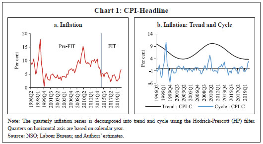 Measured (actual) inflation, however, does not fully reflect the underlying changes in the inflation process; i.e., whether the observed changes in inflation are driven by the long-term ‘trend’ component or short-term ‘cyclical’ fluctuations, which is crucial for understanding future inflation as well as the conduct of monetary policy. Trend inflation is viewed as the level to which actual inflation outcomes are expected to converge after short-run fluctuations die out (Behera and Patra, 2020), whereas the short-run fluctuations emanate from a variety of sources/price shocks mainly on the supply side. The literature suggests that under univariate framework, the overall dynamics of inflation are largely dominated by the trend component (Stock and Watson, 2007). The precise measurement of trend inflation, however, is an empirical issue (refer to Behera and Patra, op cit. for an exposition). A simple decomposition of headline inflation using the Hodrick-Prescott (HP) filter reveals that the sharp fall in trend inflation has been the driver of the general easing of headline inflation during the FIT period8. However, it can be observed that the HP trend is time-varying, while short-term fluctuations follow a stationary process (Chart 1b). In addition, short-run and long-run components of inflation are crucial in estimating inflation persistence, which has significant implications for the design of monetary policy (Ascari and Sbordone, 2014). Aggregate level analysis, however, may not fully reflect the observed changes in the volatility and persistence of the sectoral or idiosyncratic (such as food and fuel) price shocks, which are often used for calibrating model-based forecasts for policy purposes. In view of this, an analysis of the trends and cyclical components of the major groups of CPI may be necessary. It can be observed that the trend components of CPI major groups which were widely varying prior to FIT regime have become more aligned since the transition to FIT, suggesting anchoring of inflation expectations (Chart 2a). In contrast, cyclical components of inflation, which are stationary in nature, implying they even out over time, continue to exhibit significant fluctuations, albeit with some moderation in amplitudes, thus imparting volatility to actual inflation (Chart 2b). The determinants of sectoral price dynamics, therefore, should be taken into account in inflation modelling and forecasting exercises. The need for examining sectoral price dynamics may also be necessary from the perspective of understanding the sources of fluctuations in measured headline inflation, i.e., the drivers of inflation given the relative importance of food and non-food items (as represented by their weights in CPI) in the household consumption basket as well as the relative price movements over time. This is because headline inflation is derived from CPI-C, which in turn, is compiled following a bottom-up approach.9 From the monetary policy perspective, if relative price movements are large, persistent and not offsetting, they impinge on monetary policy setting as they can have a lasting influence on inflation expectations through second-round effects (RBI, 2021). 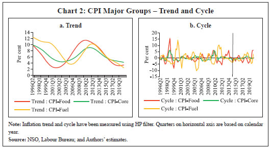 It can be observed that the food group has contributed significantly to headline inflation all through the years (Chart 3a). This is not surprising given the higher weight of food in the CPI (45.9 per cent) and frequent supply side shocks that affect food production leading to higher volatility in food prices. Food price inflation in India has also been observed to be persistent, for instance during the five-year period post-global financial crisis (GFC), reflecting a combination of supply and demand factors (Mohanty, 2014). On the other hand, the contribution of core component to CPI appears to be largely steady throughout. Moreover, relative food prices (the ratio of food to non-food price indices) trended up during 2005-2016, before showing some moderation during the FIT period reflecting record food production and improved supply management by the government (Chart 3b). Fuel (including petrol and diesel) prices, on the other hand, exhibits significant co-movement with international crude oil prices due to India’s large dependence on crude imports. Thus, given that both food and fuel prices in India are characterised by distinct inflation process (prone to supply shocks with risks of generating second round effects), aggregate level analysis may need to be strengthened with the modelling of disaggregated level inflation for generating reliable inflation forecasts for policy purposes, which is the focus of this paper. 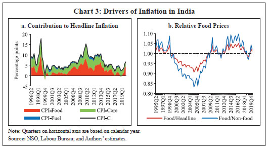 Section III
Review of Literature III.1: Time Series Models Univariate Models Many time series processes can be expressed as a parsimonious autoregressive integrated moving average (ARIMA) model after appropriate data transformation and differencing. ARIMA models employ a combination of autoregressive (past values of itself) and moving average (lagged values of a ‘white noise’ error term) models. Given the simplicity and the requirement of just one data series, ARIMA based forecasting has become one of the most common forecasting approaches. Further, by giving more weight to near-term outcomes, ARIMA models are able to beat more complicated structural models in terms of short-term forecast performance (Litterman, 1986; Stockton and Glassman, 1987; Meyler, et al. 1998). Also, unlike economic models that are restrictive in their theoretical formulations, which can inflict improper restrictions and specifications on the structural variables, ARIMA models have no such restrictions imparting the necessary flexibility to capture the dynamic properties and, thus, possess significant advantages in short-run forecasting (Saz, 2011). These models are also flexible to include deterministic effects (interventions), outliers, trading day and festival effects (Gómez and Maravall, 1998). ARIMA models can also handle seasonality in time series data and hence, forecasters give similar importance to the simplest univariate forecasting methods as econometric models. However, these models have certain drawbacks as they do not ingrain any underlying theoretical or structural relationships. ARIMA models are primarily ‘backward-looking’ which means that they are poor at predicting turning points, unless the turning point represents a return to a long-run equilibrium (Meyler, et al. 1998). Furthermore, ARIMA models are considered to be too simplistic, subjective, agnostic and atheoretic in nature (Saz, 2011). To overcome these limitations of univariate forecasting, time series models are often extended to include other variables in the form of single equation models with exogenous explanatory variables or a structural or non-structural system of equations. Multivariate Models Within multivariate models, a notable approach is to model multiple time series predictor variables simultaneously along with inflation using high-dimensional VARs (Stock and Watson, 2008; Bańbura, et al. 2010; Canova, 2011). One of the principal uses of a VAR model is to generate forecasts. These models involve constructing subsidiary models for the predictor variables, or alternatively, modelling inflation and the predictors jointly and iterating the joint model forward while imposing certain parameter restrictions which could involve complex macroeconomic structure and linkages. The merit of these models over univariate approaches is that of using additional information available from other related time series as well as theory-based structural relationships among them to obtain better forecasts. Out-of-sample forecasts are obtained via forward iteration which in practice is done by a “rolling one-period-ahead” forecast where the estimated VAR coefficients are updated each period in order to account for the latest data release of the variables. III.2: Macro-economic Models Another important modelling framework within the class of economic models is the Phillips curve10. The study of the nature of the PC trade-off has non-trivial implications for the conduct of monetary policy and business cycle fluctuations, and is routinely undertaken with the objective of modelling and forecasting inflation. The literature on PC has undergone significant changes overtime, with the New Keynesian Phillips Curve (NKPC) and its appealing theoretical microfoundations gaining popularity and becoming a standard feature of many analyses (Nason and Smith, 2008; Dees et al., 2009). The PC-based models happen to be the most widely used for inflation forecasting after the univariate approaches. III.3: The Indian Scenario Several studies have used the univariate approach to forecast inflation in the case of India. Some of the studies have used ARIMA models as benchmark to evaluate forecasting performance of their economic models (John, et al. 2020), while others, like Pratap and Sengupta (2019) have evaluated a set of models using CPI data for forecasting performance and concluded that the best forecasting performance is achieved by the SARIMA model of the form (3,1,1) (2,1,1). On the other hand, Srivastava (2016) uses ARIMA based approaches and compares direct and indirect forecasts of food inflation with the conclusion that a disaggregated approach performs better in the case of food inflation. A few papers in the Indian context have used VARs not only to estimate or determine inflation but also to study the factors that influence inflation expectations. An analysis of core inflation in a structural VAR (SVAR) framework with a vertical long-run supply curve as the identifying condition points towards the role of both demand and supply side shocks in inflation dynamics (Goyal and Pujari, 2005). The results using quarterly data from 1996-97:Q1 to 2013-14:Q3 identify crude oil price, output gap, fiscal policy and monetary policy as the determinants of inflation in India along with pointing out significant changes in India’s inflation dynamics after the global financial crisis (Mohanty and John, 2015). Further, a 7-variable SVAR framework finds evidence of inflation expectations anchoring with the Reserve Bank communications as well as headline inflation affecting inflation expectations in the short-run and core inflation dominating in the long-run (Goyal and Parab, 2019). Empirical explorations on PC in the Indian context in the last two decades have been mainly influenced by two strands of the literature: (i) The first one is an augmented PC put forth by Gordon (1998), generally referred to as the triangle model of inflation, in reference to the three basic determinants of inflation in the model – inertia, demand, and supply side factors; (ii) The second one is a modified version of the purely forward-looking NKPC (Gali and Gertler, 1999; Gali, Gertler, and Lopez-Salido, 2005). Such an ad-hoc modification was necessitated because of the lack of empirical support for the purely forward-looking NKPC as lagged inflation remained an important determinant of inflation dynamics. Consequently, a hybrid PC was born – with both forward and backward-looking components in the data generating process. While a majority of the empirical work using Indian data has been centred around these two approaches, one cannot fail to observe that there is considerable heterogeneity in the specifics of each of the studies, leading to a range of point estimates of the slope of the PC. This heterogeneity primarily arises due to the following factors: assumptions on the data generating process (inclusion/exclusion of the forward-looking component); the choice and structure of the economic activity variable [Index of Industrial Production (IIP) versus GDP]; the time period; and the specific econometric methodology used. However, despite these apparent differences, there is a general consensus on the existence of a PC relationship in the Indian scenario. Several papers have estimated the backward-looking PC similar to Gordon (1998). Using this approach on annual data from 1970-71 to 2000-01, Kapur and Patra (2000) estimate the sacrifice ratio – output forgone to achieve lower inflation – and find that lagged inflation and the demand variable, proxied by the output gap, are significant in determining inflation. Some studies using the backward-looking version of PC on annual data during 1994-2005 (Srinivasan, Mahambare and Ramachandran, 2006) and hybrid version of PC on annual data from 1996-2007 (Mishra and Mishra, 2012) find no evidence for the PC relationship, while some others find evidence for the same for the sub-sample of 2004-2009 (and not for the period 1997-2003) (Singh, Kanakaraj and Sridevi, 2011) and statistically on the borderline during the period 1996-2005 (Dua and Gaur, 2009). However, once this period of study is extended even slightly or a longer horizon is considered, the relationship comes back alive as can be found in Paul (2009), Mazumder (2011), and Patra and Kapur (2012). Similarly, Patra and Ray (2010) explore the dynamics of inflation expectations and find output gap to be one of the determinants along with lagged inflation, food and fuel price changes and real interest rate. Revisiting the PC relationship under the triangle model, Kapur (2013) concludes that the demand variable is significant even when supply shocks are not incorporated, and that rainfall shortage and minimum support price (MSP) affect inflation. Further, PC based forecasts outperform random walk model forecasts. Patra, Khundrakpam and George (2014) estimate a hybrid augmented PC and find the coefficient of output gap to be positive and significant as well as a rise in the contribution of expectations to inflation persistence, measured by the coefficient of one-period lead inflation, in the post-crisis period. Ball, Chari, and Mishra (2016) employ a backward-looking PC and explain inflation rate as a function of slow-moving average of past inflation and the deviation of output from its trend. A notable observation is that in most of the empirical work mentioned so far, inflation was represented by the WPI as the formulation of monetary policy was anchored on movements in WPI inflation11. In contrast, a number of recent papers (such as Chinoy, et al. 2016; Behera, et al. 2017; Pattanaik, et al. 2019; Sharma and Padhi, 2020; Patra, et al. 2021) have estimated similar models using the CPI based inflation in view of the switch from WPI to CPI as the inflation metric under the FIT framework in India since 2016. While Chinoy, et al. (2016) and Pattanaik, et al. (2019) explore inflation dynamics in a standard time series framework with the latter focusing exclusively on inflation expectations, Behera, et al. (2017) estimate the PC using state-level data; Sharma and Padhi (2020) propose an alternative indicator of economic slack that captures demand conditions efficiently to forecast core inflation; Patra, et al. (2021) explicitly address the time-varying and convexity properties of PC – all these papers corroborate the existing evidence on PC relationship in India. A survey on the range of point estimates of the slope coefficients and methodologies used in the literature suggests that all the studies have remained close to Gordon (1998) and Gali and Gertler (1999) in terms of the econometric methodology employed – choosing either ordinary least squares (OLS) or Instrumental Variables-Generalised Method of Moments (IV-GMM) techniques (Table 2). | Table 2: Select Studies on Phillips Curve (PC) Estimates in India (Contd.) | | Paper | Presence of PC/ Coefficient of the Output gap measure (β) | Inflation Measure/ Output gap measure | Time period/ Methodology | | Kapur and Patra (2000) | Estimates a backward-looking PC using WPI and GDP deflator; β is significant and varies in the range of 0.47 to 0.87 (for WPI) and 0.30 to 0.54 (for GDP deflator). | WPI and GDP deflator/ Real GDP gap (Using HP filter) | 1976-2001
(Annual data); OLS | | Srinivasan et al. (2006) | No evidence for PC; In some specifications, the coefficient is even negative and significant. | WPI/Index of Industrial Production (IIP) (Using HP filter) | 1994-2005
(Monthly data); OLS | | Dua and Gaur (2009) | Hybrid and backward-looking PCs; β is significant in some specifications (varies in the range of 0.10 to 0.15). | CPI/ Real GDP gap (Using HP filter) | 1996-2005
(Quarterly data); IV-GMM | | Paul (2009) | Backward-looking PC; β is significant when IIP manufacturing is used as a measure of output gap; varies in the range of 0.46 to 0.52. | WPI/ Real GDP gap, IIP gap and IIP manufacturing gap (Using HP filter) | 1956-2007
(Annual data); OLS | | Patra and Ray (2010) | Models inflation expectations in a PC framework; β is 0.14 and significant. | WPI/ Real GDP gap | 1997-2008
(Monthly data); OLS | | Singh et al. (2011) | Estimates a backward-looking PC for 1997-2003 and 2004-2009; β is significant in the latter period and varies in the range of 0.7 to 2.0. | CPI/ Real GDP gap (Using Kalman filter) | 1997-2009
(Quarterly data); OLS and IV - 2SLS | | Mazumder (2011) | Backward-looking PC; β is estimated to be 0.49 and significant. | WPI and CPI/ IIP gap (Using HP filter) | 1970-2008
(Quarterly data); OLS | | Patra and Kapur (2012) | Hybrid and backward-looking PCs; β is significant and ranges from 0.05 to 0.35. | WPI and GDP deflator/ Real GDP gap (Using HP filter) | 1997-2009
(Quarterly data); OLS and IV-GMM | | Mishra and Mishra (2012) | Hybrid PC; β is positive but not significant. | WPI/ IIP gap (Using HP filter) | 1996-2007
(Monthly data); IV-GMM | | Kapur (2013) | Backward-looking PC; β is significant and varies in the range of 0.19 to 0.30. | WPI/ Real GDP gap (Using HP filter) | 1996-2011
(Quarterly data); OLS | | Patra et al. (2014) | Hybrid PC; β is significant and varies in the range of 0.16 to 0.22. | WPI/ Real GDP gap (Using HP filter) | 1997-2012
(Quarterly data); IV-GMM | | Behera et al. (2017) | Backward-looking PC in a state-level panel framework; β is significant and varies in the range of 0.35 to 0.52. | CPI/ Real Gross State Domestic Product (GSDP gap) (Using HP filter) | 2007-2016
(Annual data); Dynamic Panel Estimation using difference/ system GMM | | Pattanaik et al. (2019) | New Keynesian PC using survey-based inflation expectations; β is significant and varies in the range of 0.25 to 0.48. | CPI/ Real GDP gap (Using HP filter) | 2008-2018
(Quarterly data); OLS | | Note: OLS: Ordinary Least Squares; IV: Instrumental Variable; 2SLS: Two-stage Least Squares; GMM: Generalised Method of Moments. | Section IV
Empirical Strategy and Estimation IV.1 Univariate Models An AR (p) process may be represented as a combination of its past values and a “white noise” error term: where εt is a white noise process with zero mean and variance σ2, B is the backshift operator and φ(B) is polynomial of degree p representing the AR terms. It models a time series as a function of its past values. Partial autocorrelation function (PACF) plots are used to take a view about the order of polynomial p. Similarly, an MA (q) process may be represented as a weighted average of a “white noise” series: where, εt is a white noise process with zero mean and variance σ2, B is the backshift operator and θ(B) is polynomial of degree q representing the MA terms. Autocorrelation function (ACF) plots are used to take a view about the order of polynomial q. When a time series is related to its past values as well as past residuals, a mixed ARMA model can satisfactorily describe it. In general, fewer parameters are required to be estimated in this case compared to a pure AR or pure MA model. An ARMA (p, q) can be represented as: A parsimonious ARMA (p, q) model may perform well in forecasting if inflation is stationary (Ang et al., 2007). In case of non-stationary series (as is the case with CPI data in India, Appendix Table A1b), an extended form of ARMA models, i.e., ARIMA, where differencing is done to make the data stationary, may describe the time series adequately. ARIMA combines autoregressive and moving average models and can be represented as:  where, εt is a white noise process with zero mean and variance σ2, B is the backshift operator, φ(B) and θ(B) are polynomials of degree p and q representing AR and MA terms, respectively, and d represents the order of integration that make the data stationary (Pankratz, 1983; Meyler, Kenny and Quinn, 1998). The ARIMA model expects the input time series to be non-seasonal or seasonally adjusted. Many time-series data, on the other hand, show seasonal fluctuations which may be used to supplement any forecasting information contained therein. The characterisation of seasonal series occurs by a strong serial correlation at the seasonal lags (of four and eight) in the case of CPI-headline and CPI-food in India (Appendix Table A2). Therefore, in this study we have attempted both ARIMA and Seasonal ARIMA (SARIMA) models to forecast inflation. SARIMA is a generalised form of ARIMA that supports the seasonal component in time series (Box and Jenkins, 1976). Researchers suggest that it may be irrational to assume the seasonal component to repeat itself in the same way cycle after cycle in practice (Özmen and Şanli, 2017). SARIMA models allow for irregularity in the seasonal pattern from one cycle to the next (Brockwell and Davis, 1991). While the process of seasonal adjustment may often be regarded as an integral part of modelling framework, there is always some loss of information from seasonal adjustment even when the seasonal adjustment process is properly conducted (IMF, 2017). Furthermore, de-seasonalising the data may remove certain peaks and troughs that may contain useful insights and may also come in conflict with economic theory (Depalo, 2009). SARIMA models thus assume significance in the forecasting literature. A SARIMA model is generally represented as SARIMA (p, d, q) (P, D, Q), with p standing for the non-seasonal autoregressive order, d standing for the non-seasonal integration order and q for the non-seasonal moving average order. In the seasonal part, P stands for the seasonal autoregressive order, D stands for the seasonal integration order, Q stands for the seasonal moving average order and m for the period or length of the season (in the monthly case 12, in the quarterly case 4). It can be expressed as follows: where, ΦP(Bm) and θQ (Bm) are polynomials of orders P and Q, respectively. There are two approaches to identify ARIMA models – the Box-Jenkins methodology and the penalty function statistics such as the Akaike Information Criterion (AIC), Schwarz Criterion (SC) and Hannan Quinn Criterion (HQC). The Box-Jenkins methodology infers the correct form of ARMA model from the sample autocorrelogram, partial autocorrelogram and inverse autocorrelogram plots. However, these plots are often difficult to interpret in the case of higher order mixed ARMA models. Additionally, presence of seasonality (Gómez and Maravall, 1998) and random noise in time series (Meyler, et al. 1998; Saz, 2011) further complicates Box-Jenkins model identification. Therefore, penalty function statistics, which is computationally simpler and objective, is often preferred for identifying ARIMA models. Accordingly, in this paper, our model identification is based on the AIC penalty function criteria (Brockwell and Davis, 1991; Burnham and Anderson, 2004). We estimate ARIMA using the maximum likelihood-based techniques on the log transformed CPI data for the sample period 1996-97:Q1 to 2017-18:Q312 and then forecast one-period ahead and four-periods ahead inflation13. We also estimate SARIMA models for the same period as an alternative to the ARIMA model to check for any improvement in the forecasting performance in view of the observed seasonality in food prices in India. The identified model satisfies the standard diagnostic checks such as autocorrelation and heteroscedasticity on residuals (Appendix Table A3). The models chosen for the headline and three major groups of CPI based on AIC are presented in Table 3. Table 3: ARIMA Models14 based on AIC
(Sample period: 1996-97:Q1 to 2017-18:Q3) | | Models | CPI-C | CPI-Core | CPI-Food | CPI-Fuel | | ARIMA | (3,1,2) | (4,1,3) | (3,1,2) | (0,1,2) | | SARIMA15 | (3,1,3)(1,0,1)4 | (2,1,0) (1,0,1)4 | (4,1,1)(0,0,1)4 | (0,1,2)(0,0,0)4 | | Source: Authors’ estimates. | IV.2 Structural Vector Auto Regression (SVAR) Models In order to introduce structural characteristics into the time series, a four variable SVAR model is estimated on quarterly data from 1996-97:Q1 to 2017-18:Q3, which apart from CPI-C/CPI-Core includes nominal exchange rate (INR-USD), real output or gross domestic product (GDP) and weighted average call money rate (WACR)16. Price of the Indian basket crude oil and absolute rainfall deviation from long period average (LPA) are incorporated as the two exogenous variables in the model given their significance in influencing India’s inflation dynamics (Chand 2010; Sonna et al. 2014; Mohanty and John 2015; Anand et al. 2016).17 All the variables, except WACR and rainfall deviation, are de-seasonalised using Census X-13ARIMA, converted to their natural logarithms, and used in their first-differenced forms [i.e., quarter-on-quarter change (q-o-q)] in the model as they are non-stationary. Stationary property of the variables is tested by employing the augmented Dickey-Fuller test of unit roots (Appendix Table A1b).18 The choice of the variables and the structural identification restrictions that the model assumes for the purpose of estimation closely resemble that in the available literature (Christiano, Eichenbaum and Evans, 1999; Kim and Roubini, 2000; Uhlig, 2005; Mohanty and John, 2015). The model adopts the following ordering of the variables {INR – USDt, GDPt, CPIt, WACRt} in their first-differenced form (barring interest rate) and uses the recursive identification method for the identifying restrictions in line with Eichenbaum and Evans (1995), and Christiano, et al. (1999).19 INR-USD exchange rate is considered to be the most pre-determined variable in the model and a shock to exchange rate impacts all the variables contemporaneously. It is assumed that the real GDP in the economy responds to exchange rate variations and crude oil price movements. Domestic price is assumed to be sensitive to exchange rate variations and changes in real GDP. The monetary policy represented by WACR responds contemporaneously to all the variables. In this type of models, it is generally assumed that the central bank of the economy looks at the current prices and output, among other indicators, when setting the monetary policy instrument at time t. The recursiveness assumption implies that exchange rate, output and prices respond only with a lag to a monetary policy shock. While such an assumption has attracted a lot of attention and debate in the literature, abandoning the assumption may also lead to a substantial cost, in the sense that the identifition of a broader set of economic relations becomes complicated (Christiano, et al. 1999). Accordingly, let Yt denote a k X 1 vector of {INR – USDt, GDPt, CPIt, WACRt} at time t. Considering the structural identifying restrictions stated above, the model in a VAR framework can be written as: where, ut is a k X 1 vector of structural shocks following N = (0,Σ); Σ = diag (σj); Fi is a (k X k) matrix of parameters for 1, 2 ,...,s; while matrix A is the contemperaneous matrix (Fo) For identifying the above model, k(k + 1)/2 restrictions are required to be imposed on A matrix, of which k restrictions could be satisfied by normalising the diagonal elements of A to unity. In our model k = 4. Therefore, we need to impose 6 additional restrictions on the contemporaneous correlations for identification of the four structural shocks (exchange rate shock, output shock, price shock and monetary policy shock). This is done by specifying A as a lower triangular matrix. where, Bi = A-1 Fi and εt follows N = (0,I). This model is estimated on two measures of inflation: Model 1 with CPI-C as the headline inflation measure and Model 2 with CPI excluding food and fuel as the measure of core inflation. The lag lengths for the models are chosen based on the AIC and SC criteria. The models satisfy the stability test (roots of characteristic polynomial were inside the unit circle) as well as the residual autocorrelation test (Appendix Tables A4.1 and A4.2). The structural impulse response functions (IRFs) of inflation with respect to the exchange rate shock, output shock and policy rate shock broadly meet our expectations (Chart 4). On transformation [of standard error (SE) shock to equivalent per cent], a one per cent appreciation of the exchange rate leads to a fall in headline inflation (core inflation) by 12 basis points (bps) (9 bps) in the first quarter itself20; a one per cent increase in output pushes up headline inflation (core inflation) by 27 bps (28 bps) accumulated over the first two quarters, with the peak impact of 22 bps (18 bps) in the second quarter; while the impact of policy rate changes on inflation lasts longer – a one per cent increase in interest rate results in a fall in headline inflation (core inflation) by 15 bps (16 bps) in the second quarter and a cumulative fall of 50 bps (35 bps) over a span of 3 years (Appendix Table A5). The IRFs also indicate that the impact of an interest rate shock on inflation is highly persistent as compared to the exchange rate shock and output shock.21 Further, in terms of the channel via which policy rate shock impacts inflation, the IRFs suggest that the impact is via output, where a positive policy rate shock leads to a fall in output (Appendix Charts A.1 and A.2)22. 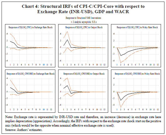 In order to quantify the relative importance of various shocks in explaining the fluctuations in inflation, a variance decomposition analysis was conducted. The results show that the fluctuations in inflation is explained mostly by its own shock. Among the other shocks, the policy rate shock is most important explaining about 7-9 per cent of the variance in inflation over the medium term, as compared to about 2-4 per cent in case of exchange rate and output. Thus, the variance decomposition analysis along with impulse response functions clearly point out the significance of policy rate shock over exchange rate and output shocks for both headline inflation and core inflation in India (Appendix Table A6). IV.3 Phillips Curve (PC) Based Models In this section, inflation dynamics is modelled in three ways: the backward-looking triangle model of Gordon (1998); a purely forward-looking NKPC; and a hybrid NKPC which incorporates forward and backward-looking components similar to Gali and Gertler (1999), Patra and Kapur (2012) and Patra, et al. (2014). More precisely, we estimate the following specifications:  where, πt is a measure of inflation, Xt is a measure of economic activity represented by output gap [(actual output minus potential output23/potential output)*100], Δ stands for first difference, and Zt is a vector of supply side factors; Etπt+1 is the expected future inflation and εt is the white noise term (refer to Appendix Table A1a for a detailed description of variables). In equation (10), the coefficients of the inflation terms on the right-hand side are restricted to sum up to unity24, implying the existence of a vertical long-run Phillips curve. All variables, except minimum support prices (MSP) and absolute rainfall deviation from LPA (part of the Z vector), are deseasonalised using Census X-13ARIMA. The presence of unit roots in the variables is tested by employing the augmented Dickey-Fuller test and the test results are presented in the Appendix Table A1b. The difference between the PC specifications in (8), (9) and (10) and the standard ones generally found in extant literature in the Indian context is the presence of the additional term Δ Xt-1 – change in output gap – which is included to capture the possibility of speed limit effects (Fisher, Mahadeva and Whitley, 1997; Gruen, Pagan and Thompson, 1999; Malikane, 2014). The speed limit gets its name from the suggestion that more rapid changes in economic activity may cause larger changes in the inflation rate for a given level of the economic activity (Fuhrer, 1995). The coefficients, β1 and β2, therefore provide measures of the flexibility in price adjustment. Equations (8), (9) and (10) are estimated on quarterly data for the sample period 1996-97:Q1 to 2017-18:Q3 with q-o-q change in headline CPI as well as its major components – core, food and fuel – as dependent variables, using OLS method. Even though PC estimation is typically undertaken using headline or core inflation as the inflation metric, we delve into other major sub-components (food and fuel) for two reasons: first, to understand the drivers of sub-component level inflation dynamics; and second, to generate inflation forecasts from the indirect approach to compare with aggregate level inflation forecast, given the focus of the paper in generating inflation forecasts while capturing the changes in the inflation process. Furthermore, the final form of the equations is derived by starting with a general form with several lags of the output gap and choosing an appropriate model based on the significance of relevant coefficients and overall fit. The results are given in Tables 4, 5, 6 and 7, respectively. Two variables are used to capture inflation expectations Etπt+1 – the lead q-o-q change in headline CPI (in specification 2) and the lagged headline trend25 (q-o-q) (in specifications 3 and 4) in Table 4. Trend headline inflation can be used as a proxy for expected inflation: (i) as inflation outcome is expected to converge to its trend after the shocks to inflation die out (Behera and Patra, 2020) and (ii) as a substantial portion of observed inflation persistence can be attributed to variation in trend inflation, which in turn is related to changes in monetary regimes (Garnier et al., 2015). Moreover, there was no unique inflation target for the whole sample period (there was a change in the inflation metric for policy from WPI to CPI with the adoption of FIT) which could be used as a proxy for inflation expectations. As can be observed, the leads and lags of price changes are generally significant. The coefficient of lagged headline CPI trend26 is greater compared to lag of headline CPI q-o-q change (Table 4, specification 4), indicating its relative importance in determining inflation dynamics in India. The coefficients of the measure of economic activity – real output gap (7 quarters before) and the change in real output gap (1 quarter before) – are both positive and significant in all the specifications suggesting that demand factors play an important role in determining inflation in India. In other words, inflation depends as much on the change in output gap as on the level implying the presence of speed limit effects. However, the less than proportional impact of output gap on inflation (the lower coefficients) indicates lower degree of flexibility in price adjustment. Other variables that affect headline inflation are MSP, exchange rate and global non-fuel inflation. | Table 4: Headline CPI (q-o-q change in per cent) | | | (1) | (2) | (3) | (4) | Headline
(Triangle Model) | Headline
(NKPC) | Headline
(NKPC 2) | Headline
(Hybrid) | | ΔCPICt–1 | 0.214** | - | - | 0.000890 | | (0.106) | | | (0.109) | | ΔCPIt+1 | - | 0.389*** | - | - | | | (0.116) | | | | Inflation trendt–1 | | | 1.030*** | 0.999*** | | - | - | (0.227) | (0.109) | | Output gapt–7 | 0.150* | 0.197** | 0.218*** | 0.217*** | | (0.0831) | (0.0788) | (0.0747) | (0.0760) | | ΔOutput gapt–1 | 0.205** | 0.241*** | 0.191** | 0.191** | | (0.0943) | (0.0899) | (0.0849) | (0.0848) | | MSP variationt–1 | 0.0480* | 0.0214 | -0.00548 | -0.00356 | | (0.0243) | (0.0252) | (0.0256) | (0.0213) | | ΔExchange ratet–1 | 0.0819* | 0.0785* | 0.0620 | 0.0634 | | (0.0448) | (0.0415) | (0.0396) | (0.0394) | | ΔGlobal nonfuel pricet–1 | 0.0482* | 0.0585** | 0.0458** | 0.0463* | | (0.0263) | (0.0237) | (0.0227) | (0.0234) | | Rainfall deviationt–2 | 0.00174 | -0.00403 | 0.0000645 | 0.000125 | | (0.00682) | (0.00676) | (0.00616) | (0.00614) | | 27R2 | 0.521 | 0.564 | 0.611 | - | | N | 80 | 80 | 80 | 80 | | Portmanteau test for white noise (Q statistic p-value) | 0.8503 | 0.8885 | 0.9637 | 0.9606 | Notes: ‘Inflation trend’ is constructed by applying the HP filter on the CPI headline q-o-q series. Specifications 1-4 include the following quarter dummy variables – 1998q4; 1999q1; 2000q3; 2005q4; and 2012q2. Exchange rate is represented by INR-USD rate and therefore, an increase (decrease) in exchange rate here implies depreciation (appreciation).
Standard errors in parentheses.
* p < 0.10, ** p < 0.05, *** p < 0.01
Source: Authors’ estimates. |
| Table 5: Core CPI (q-o-q change in per cent) | | | (1) | (2) | (3) | (4) | CPI Core
(Triangle Model) | CPI Core
(NKPC) | CPI Core
(NKPC 2) | CPI Core
(Hybrid) | | ΔCPI Coret–1 | 0.187* | - | - | 0.00989 | | (0.0941) | | | (0.108) | | ΔCPI Coret+1 | - | 0.242** | - | - | | | (0.116) | | | | Inflation trendt–1 | - | - | 0.707*** | 0.990*** | | | | (0.181) | (0.108) | | Output gapt–7 | 0.161** | 0.183*** | 0.152** | 0.142** | | (0.0627) | (0.0679) | (0.0638) | (0.0646) | | ΔOutput gapt–1 | 0.224*** | 0.277*** | 0.208** | 0.198** | | (0.0808) | (0.0887) | (0.0805) | (0.0827) | | ΔExchange ratet–1 | 0.0653* | 0.0617* | 0.0438 | 0.0321 | | (0.0359) | (0.0349) | (0.0331) | (0.0330) | | ΔIndbasket crudet–1 | 0.00811 | 0.00849 | 0.00702 | 0.00696 | | (0.00560) | (0.00614) | (0.00572) | (0.00583) | | R2 | 0.550 | 0.431 | 0.501 | - | | N | 80 | 80 | 80 | 80 | | Portmanteau test for white noise (Q statistic p-value) | 0.3757 | 0.5816 | 0.1835 | 0.2395 | Notes: ‘Inflation trend’ is constructed by applying the HP filter on CPI headline (q-o-q change). Specification 1 includes the following quarter dummy variables – 1998q3; 2005q1; 2009q4; 2010q1; and 2012q1. Specifications 2-4 include the following quarter dummy variables – 2009q4; and 2010q1. Exchange rate is represented by INR-USD rate and therefore, an increase (decrease) in exchange rate here implies depreciation (appreciation).
Standard errors in parentheses.
* p < 0.10, ** p < 0.05, *** p < 0.01
Source: Authors’ estimates. | Similar to the headline specification, Etπt+1 in the case of core is captured by two variables – lead core q-o-q inflation (specification 2 in table 5) and lagged q-o-q inflation trend derived from headline (specifications 3 and 4). The lags and leads of price changes are significant here too. Besides, the coefficient of lagged headline trend is greater compared to lag of core q-o-q inflation (Table 5, specification 4) as was the case in headline. The coefficients of the level as well as change in the output gap are statistically significant and positive, corroborating the speed limit effects. | Table 6: Food CPI (q-o-q change in per cent) | | | (1) | (2) | (3) | | CPI Food | CPI Food | CPI Food | | ΔCPI Foodt–1 | 0.271*** | - | 0.180** | | (0.0866) | - | (0.0867) | | Inflation trendt–1 | - | 1.532*** | 0.820*** | | | (0.361) | (0.0867) | | MSP variationt–1 | 0.0824** | 0.0114 | 0.0392 | | (0.0313) | (0.0368) | (0.0286) | | Rainfall deviationt–2 | 0.0166* | 0.0169* | 0.0163* | | (0.00944) | (0.00900) | (0.00889) | | ΔGlobal foodpricet–1 | 0.0159 | 0.0473 | 0.0304 | | (0.0319) | (0.0306) | (0.0302) | | R2 | 0.543 | 0.583 | - | | N | 87 | 87 | 87 | | Portmanteau test for white noise (Q statistic p-value) | 0.1962 | 0.5367 | 0.3371 | Notes: ‘Inflation trend’ is constructed by applying the HP filter on CPI headline (q-o-q change). Specifications here include the following quarter dummy variables – 1998q1; 1998q4; 1999q1; 2006q2; 2010q4; 2011q1; and 2011q1.
Standard errors in parentheses.
* p < 0.10, ** p < 0.05, *** p < 0.01
Source: Authors’ estimates. | Food inflation is modelled in a similar fashion except that it leaves out the output gap variable, as food prices are determined more by supply side factors, given the broadly inelastic nature of food demand28. MSP and rainfall deviation influence food inflation significantly and positively, apart from the lags of inflation. Once again, the lagged headline CPI trend is highly significant, and the magnitude of its coefficient is comparatively higher (Table 6). Analogously, output gap variables are omitted in the case of fuel inflation as well. The results show that fuel inflation (q-o-q change) is significantly and positively influenced by crude oil inflation. Moreover, identical inferences can be made with regard to lagged headline CPI trend (Table 7). | Table 7: Fuel CPI (q-o-q change in per cent) | | | (1) | (2) | (3) | | CPI Fuel | CPI Fuel | CPI Fuel | | ΔCPI Fuelt–1 | 0.156*** | - | 0.149*** | | (0.0571) | | (0.0562) | | Inflation trendt–1 | | 0.576** | 0.851*** | | - | (0.230) | (0.0562) | | ΔIndbasket crudet–1 | 0.0214*** | 0.0219*** | 0.0209*** | | (0.00754) | (0.00769) | (0.00741) | | ΔIndbasket crudet–2 | - | 0.00661 | - | | | (0.00712) | | | ΔExchange ratet–1 | 0.0551 | 0.0583 | 0.0199 | | (0.0402) | (0.0410) | (0.0391) | | R2 | 0.756 | 0.757 | - | | N | 90 | 89 | 90 | | Portmanteau test for white noise (Q statistic p-value) | 0.8643 | 0.1340 | 0.3172 | Notes: ‘Inflation trend’ is constructed by applying the HP filter on the CPI headline q-o-q series. Specifications here include the following quarter dummy variables – 2000q2; 2000q4; 2002q1; 2005q2; 2010q3; and 2011q1. Exchange rate is represented by INR-USD rate and therefore, an increase (decrease) in exchange rate here implies depreciation (appreciation).
Standard errors in parentheses.
* p < 0.10, ** p < 0.05, *** p < 0.01
Source: Authors’ estimates. | The Reserve Bank has been collecting 3-months ahead and 1-year ahead inflation expectations of households through quarterly surveys since 2005. Similar to the analysis undertaken in Pattanaik, et al. (2019), we use these survey-based inflation expectations in an NKPC framework for a truncated sample period (and find the results to be qualitatively similar to that of the longer time period discussed in this section (Appendix Table A7) – inflation expectations (both 3-months and 1-year ahead) and output gap are signficant in determining inflation. These results are also in line with Pattanaik, et al. (2019). As a robustness check, these specifications were estimated using IV-GMM as well, and the results were found to be broadly similar (Appendix Tables A8 and A9). Section V
Evaluating Forecasting Performance Given the objective of this paper, an evaluation of the forecasting performance is done based on the root mean square errors (RMSEs) and mean absolute errors (MAEs) calculated by comparing the derived y-o-y inflation forecasts generated from these alternative models discussed in section IV with the actual y-o-y inflation.29 Additionally, in line with the literature, we also provide forecasts generated from a random walk model as a benchmark30. We do not go into forecasting inflation at a disaggregated level in the case of SVAR because these models are generally backed by economic theories and linkages that largely work at the macro-level. Moreover, literature also tends to use SVAR models more on validating and establishing larger macroeconomic theories. In the case of PC models, headline and core inflation forecasts are based on specifications (1), (3) and (4) in Tables 4 and 5 – i.e., we do not employ specification 2 in which inflation expectations are captured through lead headline (core) inflation, as it is useful for modelling but not amenable for out-of-sample forecasting. As discussed earlier, a key objective here is to evaluate the merit of a disaggregated approach; we, therefore, compare the forecasts of headline inflation obtained directly and indirectly (a weighted average31 of the forecasts of the three sub-components – core, food and fuel – based on their fixed weights in the CPI-C). Forecast periods are restricted to 2017-18:Q4 to 2019-20:Q4 (9 quarters) for one-period ahead and 2018-19:Q3 to 2019-20:Q4 (6 quarters) for four-periods ahead inflation forecasts to allow forecast comparison over a reasonably long period. The results indicate that SARIMA outperforms both SVAR and PC models in one period ahead headline forecasts, reflecting gains from flexibility as there are no restrictions (unlike the economic models) to capture the dynamic properties (Litterman, 1986; Stockton and Glassman, 1987). Secondly, in the case of one-period ahead ARIMA forecasting, direct forecasts perform better than indirect ones (sum of component forecasts), indicating that noise associated with volatile food and fuel groups plausibly contaminates the aggregation of forecasts (Table 8). This is in line with the findings of Pratap and Sengupta (2019) for India. Along similar lines, many other studies have concluded that disaggregation does not necessarily imply forecast improvement (Benalal, Diaz del Hoyo, Landau, Roma and Skudelny, 2004; Hubrich, 2005; Cushing, 2014). Finally, while a simple ARIMA on core is better, SARIMA models are better in the case of headline primarily indicating the existence of seasonality in food prices that is captured in headline inflation. An assessment of four-periods ahead forecasts, however, suggests that the PC-based models (NKPC and hybrid NKPC) perform better than ARIMA/SARIMA models in the case of CPI core; in the case of headline, NKPC and hybrid NKPC outperform every model apart from SARIMA under direct approach (Table 9). Although SVAR model may be capturing the structural dynamics factoring in the role of policy variable, it falls behind PC models in forecasting inflation, which better captures the role of expectations in determining the inflation dynamics in India. | Table 8: One Period Ahead Forecasts: 2017-18:Q4 to 2019-20:Q4 (9 Quarters) | | Models | CPI – Direct | CPI Core | CPI C – Indirect | | RMSE | MAE | RMSE | MAE | RMSE | MAE | | Random Walk | 1.02 | 0.75 | 0.62 | 0.51 | 1.03 | 0.76 | | ARIMA | 0.81 | 0.70 | 0.45 | 0.38 | 0.86 | 0.74 | | SARIMA | 0.64 | 0.49 | 0.48 | 0.37 | 0.85 | 0.72 | | SVAR | 0.77 | 0.72 | 0.69 | 0.52 | _ | _ | | Phillips Curve (PC) Models | | | | | | | | Model 1 – Backward-looking PC | 1.22 | 1.06 | 0.52 | 0.39 | 1.17 | 1.01 | | Model 2 – NKPC (with lagged trend inflation) | 0.94 | 0.75 | 0.45 | 0.38 | 0.92 | 0.75 | | Model 3 – Hybrid NKPC (with the constraint) | 0.96 | 0.78 | 0.47 | 0.43 | 0.90 | 0.70 | | Source: Authors’ estimates. |
| Table 9: Four-Periods Ahead Forecasts: 2018-19:Q3 to 2019-20:Q4 (6 Quarters) | | Models | CPI C – Direct | CPI Core | CPI C – Indirect | | RMSE | MAE | RMSE | MAE | RMSE | MAE | | Random Walk | 2.57 | 2.27 | 1.54 | 1.36 | 2.55 | 2.27 | | ARIMA | 2.82 | 2.35 | 1.88 | 1.76 | 2.92 | 2.46 | | SARIMA | 1.42 | 1.29 | 1.91 | 1.79 | 2.93 | 2.47 | | SVAR | 2.32 | 2.00 | 2.40 | 2.25 | _ | _ | | Phillips Curve (PC) Models | | | | | | | | Model 1 – Backward-looking PC | 3.80 | 3.23 | 2.10 | 2.07 | 3.19 | 2.69 | | Model 2 – NKPC (with lagged trend inflation) | 1.78 | 1.67 | 1.00 | 0.82 | 1.58 | 1.49 | | Model 3 – Hybrid NKPC (with the constraint) | 1.78 | 1.66 | 0.74 | 0.68 | 1.71 | 1.67 | | Source: Authors’ estimates. | Furthermore, we employ a formal test for comparing forecast accuracy – the Diebold-Mariano (DM) test (Diebold and Mariano, 1995). The null hypothesis of the DM test is that the forecast accuracy of any given two models is equal. We find that direct forecast outperforms the indirect forecast in the case of univariate models both for one-quarter and four-quarters ahead horizons; while in the case of PC-based models, indirect forecasts are generally better compared to direct forecasts32. These findings indicate that apart from aggregate forecast, disaggregated forecasts may also be useful from the perspective of four-quarters ahead inflation forecasting under different PC models, which better capture the varying properties of the data generating processes of the sub-components of CPI-C in India, which is not possible to capture simply by its own past as in ARIMA models. However, over one-quarter ahead horizon, inflation model based on the behaviour of past inflation alone produces the best forecast. On the other hand, despite poor performance of SVAR models in forecasting, impulse-responses from these models provide useful insights in identifying the direction of linkages and the impact of shocks, which are important in policy analysis and therefore, should be a part of any modelling and forecasting exercise of inflation. Section VI
Conclusion Under a flexible inflation targeting monetary policy framework, inflation forecast acts as the intermediate target. Therefore, generating accurate, reliable and unbiased inflation forecasts for the conduct of monetary policy assumes significance. Forecast accuracy helps in the optimal conduct of monetary policy and thereby promotes policy credibility. This paper models and forecasts CPI inflation using both univariate and multivariate models following two approaches – direct (based on aggregate data) and indirect (based on disaggregate data, i.e., major components of CPI, which are then combined). It corroborates the existence of a PC relationship in India and finds that the dynamics of sub-components of CPI-C are different. While output gap and exchange rate affect core inflation, changes in MSP and rainfall deviation influence food inflation. Fuel inflation is mainly determined by international crude oil prices. Notwithstanding the varying dynamics at the disaggregated level, forecasts generated using the indirect approach do not perform as well as the univariate forecasts at the aggregate level. Furthermore, simple univariate models produce better forecasts compared to structural multivariate models for the one-quarter ahead forecast horizon. For four-quarters ahead forecasts horizon, however, the PC-based models outperform others in the case of CPI core; in the case of headline, they outperform every model apart from SARIMA under direct approach. Further, PC-based forecasts generated via the indirect approach is better than those generated through the direct approach, indicating that disaggregated level dynamics of inflation could also be useful for generating inflation projections in India. The question on suitability of direct versus indirect forecasts, thus, crucially depends on the forecast horizon and the underlying model. SVAR models, despite having poor forecast performance, provide valuable insights for evaluating the impact of shocks, which are useful from the perspective of policy analysis. As a way forward, inflation forecasting models based on time-varying parameter VAR combined with stochastic volatility may be considered to take into account the changing inflation dynamics over time driven by both structural changes taking place in the economy and shifts in policy regimes.
References Anand, R., Kumar, N., & Tulin, V. (2016). Understanding India’s food Inflation: The role of demand and supply factors. IMF Working Paper WP/16/2. Ang, A., Bekaert, G., & Wei., M. (2007). Do macro variables, asset markets, or surveys forecast inflation better?. Journal of Monetary Economics, 54, 1163-1212. Ascari, G., & Sbordone, A. M. (2014). The macroeconomics of trend inflation. Journal of Economic Literature, 52(3), 679-739. Atkeson, A., & Ohanian, L. (2001). Are Phillips curves useful for forecasting inflation? Quarterly Review of Federal Reserve Bank of Minneapolis, 25, 2-11. Ball, L., Chari, A., & Mishra, P. (2016). Understanding Inflation in India. NBER Working Paper Series, No. w22948. Bańbura, M., Giannone, D., & Reichlin, L. (2010). Large Bayesian VARs. Journal of Applied Econometrics, 25(1), 71-92. Barnett, W. A., Bhadury, S. S., & Ghosh, T. (2016). An SVAR approach to evaluation of monetary policy in India: Solution to the exchange rate puzzles in an open economy. Open Economies Review, 27(5), 871-893. Behera, H. K., & Patra, M. D. (2020). Measuring trend inflation in India. RBI Working Paper Series: 15/2020. Behera, H., Wahi, G., & Kapur, M. (2017). Phillips Curve relationship in India: Evidence from state-level analysis. RBI Working Paper Series: 08/2017. Benes, J., Clinton, K., George, A. T., John, J., Kamenik, O., Laxton, D., .. Zhang, F. (2016). Inflation-forecast targetig for India: An outline of the analytical framework. RBI Working Paper Series: 07/2016. Bhattacharya, R., Patnaik, I., & Shah, A. (2008). Exchange rate pass-through in India. New Delhi: National Institute of Public Finance and Policy. Blanchard, O., Cerutti, E., & Summers., L. (2015). Inflation and activity–two explorations and their monetary policy implications. National Bureau of Economic Research, No. w21726. Blinder, A. S. (2018). Is the Phillips curve dead? And other questions for the Fed. Wall Street Journal, May 3. Box, G., & Jenkins, G. (1976). Time Series Analysis: Forecasting and Control. Holden Day: San Francisco. Brockwell, P., & Davis, R. (1991). Time Series: Theory and Methods. New York: Springer, 2nd edition. Burnham, K. P., & Anderson, D. R. (2004). Multimodel inference: understanding AIC and BIC in model selection. Sociological methods & research, 33(2), 261-304. Canova, F. (2011). Methods for applied macroeconomic research. Princeton university press. Chand, R. (2010). Understanding the nature and causes of food inflation. Economic and Political Weekly, XLV (9), 10-13. Chinoy, S. Z., Kumar, P., & Mishra, P. (2016). What is responsible for India’s sharp disinflation?. In Monetary Policy in India (pp. 425-452). Springer, New Delhi. Christiano, L. J., Eichenbaum, M., & Evans, C. L. (1999). Monetary policy shocks: What have we learned and to what end?. Handbook of macroeconomics, 1, 65-148. Coibion, O., & Gorodnichenko, Y. (2015). Is the Phillips curve alive and well after all? Inflation expectations and the missing disinflation. American Economic Journal: Macroeconomics, 7(1),197-232. Cushing, S. K. (2014). Does using disaggregate components help in producing better forecasts for aggregate inflation. Journal of Economics and Development Studies, 2(2), 527-546. Das, S. (2020). Seven Ages of India’s Monetary Policy. Address delivered at the St. Stephen’s College, University of Delhi on January 24, 2020. Dees, S., Pesaran, M. H., Smith, L. V., & Smith, R. P. (2009). Identification of new Keynesian Phillips curves from a global perspective. Journal of Money, Credit and Banking, 41(7), 1481-1502. Depalo, D. (2009). A seasonal unit-root test with Stata. The Stata Journal, 9(3), 422–438. Dholakia, R. H., & Kandiyala, V. S. (2018). Changing dynamics of inflation in India. Economic and Political Weekly, 65-73. Diebold, F. M., & Mariano, R. (1995). Comparing predictive accuracy. Journal of Business & economic statistics, 13(3). Dua, P., & Gaur, U. (2009). Determination of inflation in an open economy phillips curve framework: The case of developed and developing asian countries. Working paper 178, Centre for Development Economics; Delhi School of Economics. Duncan, R., & Martínez-García, E. (2015). Forecasting local inflation with global inflation: When economic theory meets the facts. Globalization and Monetary Policy Institute Working Paper, (235). Duncan and Martínez-García. (2019). New perspectives on forecasting inflation in emerging market economies: An empirical assessment. International Journal of Forecasting, 35(3), 1008-1031. Eichenbaum, M., & Evans, C. L. (1995). Some empirical evidence on the effects of shocks to monetary policy on exchange rates. The Quarterly Journal of Economics, 110(4), 975-1009. Fisher, P. G., Mahadeva, L., & Whitley., J. D. (1997). The output gap and inflation–Experience at the Bank of England. BIS Conference Papers, Vol. 4. Fuhrer, J. C. (1995). The Phillips curve is alive and well. New England Economic Review, 41-57. Gali, J., & Gertler, M. (1999). Inflation dynamics: A structural econometric analysis. Journal of Monetary Economics, 44(2), 195-222. Gali, J., Gertler, M., & Lopez-Salido, D. (2005). Robustness of the estimates of the hybrid New Keynesian Phillips curve. Journal of Monetary Economics, 52(6), 1107–1118. Garnier, C., Mertens, E., & Nelson, E. (2015). Trend inflation in Advanced Economies. International Journal of Central Banking, 11(4), 65-136. Gómez, V., & Maravall, A. (1998). Automatic modelling methods for univariate. Banco de España Working Paper No. 9808. Gordon, R. J. (1998). Foundations of the Goldilocks economy: supply shocks and the time-varying NAIRU. Brookings Papers on Economic Activity, 1998(2), 297-346. Goyal, A., & Parab, P. (2019). Modelling heterogeneity and rationality of inflation expectations across indian households. IGIDR Working Paper WP-2019-002. Goyal, A., & Pujari, A. K. (2005). Analysing Core Inflation in India: A Structural VAR Approach. Retrieved from https://mpra.ub.uni-muenchen.de/67105/1/MPRA_paper_67105.pdf Gruen, D., Pagan, A., & Thompson., C. (1999). The phillips curve in Australia. Journal of Monetary Economics, 44(2), 223-258. Hendry, D. F., & Hubrich, K. (2006). Forecasting economic aggregates by disaggregates. ECB Working Paper Series (No. 589). Hubrich, K. (2005). Forecasting euro area inflation: Does aggregating forecasts by HICP component improve forecast accuracy? European Central Bank, Research Department, 21(1), 119– 136. Huwiler, M., & Kaufmann, D. (2013). Combining disaggregate forecasts for inflation: The SNB’s ARIMA model. Swiss National Bank Economic Studies, (7). IMF. (2017). Quarterly National Accounts Manual: Chapter 7 - Seasonal Adjustment. Iyer, T., & Gupta, A. S. (2019). Quarterly forecasting model for india’s economic growth: Bayesian Vector Autoregression Approach. Asian Development Bank Economics Working Paper Series, (573). John, J., Singh, S., & Kapur, M. (2020). Inflation forecast combinations – The Indian experience. RBI Working Paper Series: 11/2020. Kabukçuoğlu, A., & Martínez-García, E. (2018). Inflation as a global phenomenon—Some implications for inflation modeling and forecasting. Journal of Economic Dynamics and Control, 87, 46-73. Kapur, M. (2013). Revisiting the Phillips curve for India and inflation forecasting. Journal of Asian Economics, 25, 17-27. Kapur, M., & Patra, M. D. (2000). The Price of Low Inflation. Reserve Bank of India Occasional Papers, 21(2), 191-234. Kim, S., & Roubini, N. (2000). Exchange rate anomalies in the industrial countries: A solution with a structural VAR approach. Journal of Monetary economics, 45(3), 561-586. Litterman, R. B. (1986). Forecasting with Bayesian vector autoregressions—five years of experience. Journal of Business & Economic Statistics, 4(1), 25-38. Malikane, C. (2014 ). A new Keynesian triangle Phillips curve. Economic Modelling 43, 247-255. Mandalinci, Z. (2017). Forecasting inflation in emerging markets: An evaluation of alternative models. International Journal of Forecasting, 33(4), 1082-1104. Mathai, K. (2009). Back to basics: What is monetary policy?. Finance & Development, 46(003). Mazumder, S. (2011). The stability of the Phillips curve in India: Does the Lucas critique apply? Journal of Asian Economics, 22(6), 528-539. Meyler, A., Kenny, G., & Quinn, T. (1998). Forecasting irish inflation using ARIMA models. Central Bank and Financial Services Authority of Ireland Technical Paper Series, 1-48. Mishra, A., & Mishra, V. (2012). Evaluating inflation targeting as a monetary policy objective for India. Economic Modelling, 29(4), 1053–1063. Mohanty, D. (2014). Why is recent food inflation in India so persistent? Annual Lalit Doshi Memorial Lecture, St. Xavier’s College, Mumbai. Mohanty, D., & John, J. (2015). Determinants of inflation in India. Journal of Asian Economics, 36, 86-96. Nason, J. M., & Smith, G. W. (2008). Identifying the new Keynesian Phillips curve. Journal of Applied Econometrics, 23(5), 525-551. Benalal, N., Diaz del Hoyo, J. L., Landau, B., Roma, M., & Skudelny, F. (2004). To aggregate or not to aggregate? Euro area inflation forecasting. Euro Area Inflation Forecasting (July 2004). Ouliaris, S., Pagan, A., & Restrepo, J. (2016). Quantitative macroeconomic modeling with structural vector autoregressions–an Eviews implementation. IHS Global, 13. Özmen, M., & ŞANLI, S. (2017). Detecting the best seasonal Arima forecasting model for monthly inflation rates in Turkey. Dokuz Eylül Üniversitesi İktisadi İdari Bilimler Fakültesi Dergisi, 32(2), 143-182. Pankratz, A. (1983). Forecasting with Univariate Box-Jenkins Models: Concepts and Cases. John Wily & Sons. Patra, M. D., & Kapur, M. (2012). A monetary policy model for India. Macroeconomics and finance in emerging market economies, 5(1), 18-41. Patra, M. D., & Ray, P. (2010). Inflation expectations and monetary policy in India: An Empirical Exploration. IMF Working Paper (WP/10/84). Patra, M. D., Behera, H., & John, J. (2021). Is the Phillips curve in India dead, inert and stirring to life or alive and well? RBI Bulletin, November, 63-75. Patra, M. D., Khundrakpam, J. K., & George, A. T. (2014). Post-Global crisis inflation dynamics in India: What has changed? In S. Shah, B. Bosworth, & A. Panagariya, India Policy Forum 2013-14 (pp. 117-191). New Delhi; Washington DC: Sage publications. Patra, M.D., Khundrakpam J. K., and John, J. (2018). Non-linear, asymmetric and time-varying exchange rate pass-through: Recent evidence from India. RBI Working Paper Series: 02/2018. Pattanaik, S., Muduli, S., & Ray, S. (2019). Inflation expectations of households: Do they influence wage-price dynamics in India? RBI Working Paper Series: 01/2019. Paul, B. P. (2009). In search of the Phillips curve for India. Journal of Asian Economics, 20(4), 479–488. Phillips, A. W. (1958). The relation between unemployment and the rate of change of money wage rates in the United Kingdom, 1861-1957. Economica, 25(100), 283-299. Pincheira, P., & Medel, C. (2012). Forecasting inflation with a random walk. Bank of Chile Working Paper No. 669. Pratap, B., & Sengupta, S. (2019). Macroeconomic forecasting in india:does machine learning hold the key to better forecasts? RBI Working Paper Series: 04/2019. Raj, J., Kapur, M., George, A., Wahi, G., & Kumar, P. (2019). Inflation forecasts: Recent experience in India and a cross-country assessment. The Reserve Bank of India Mint Street Memo No. 19, May. RBI. (2021). Report on Currency and Finance 2020-21: Reviewing the Monetary Policy Framework. Saz, G. (2011). The efficacy of SARIMA models for forecasting inflation rates in developing countries: The case for Turkey. International Research Journal of Finance and Economics, 62, 111-142. Sharma, S., & Padhi, I. (2020). An alternative measure of economic slack to forecast core inflation. Reserve Bank of India Occasional Papers, 41(2). Singh, B. K., Kanakaraj, A., & Sridevi, T. (2011). Revisiting the empirical existence of the Phillips curve for India. Journal of Asian Economics, 22(3), 247-258. Sonna, T., Joshi, H., Sebastian, A., & Sharma, U. (2014). Analytics of food inflation in India. RBI Working Paper Series: 10/2014. Srinivasan, N., Mahambare, V., & Ramachandran, M. (2006). Modelling inflation in India: A critique of the structuralist approach. Journal of Quantitative Economics, 4(2), 45-58. Srivastava, S. K. (2016). Short run forecast of food inflation using ARIMA: A combination approach. In Analytical Techniques for Decision Making in Agriculture. (pp. 82-92). Daya Publishing House. Stock, J. H., & Watson, M. M. (2008). Phillips curve inflation forecasts. NBER Working Paper (w14322). Stock, J. H., & Watson, M. W. (2007). Why has US inflation become harder to forecast?. Journal of Money, Credit and Banking, 39, 3-33. Stock, J. H., & Watson, M. W. (2010). Modeling inflation after the crisis. NBER Working Paper, No. w16488. Stockton, D. J., & Glassman, J. E. (1987). An evaluation of the forecast performance of alternative models of inflation. The review of economics and statistics, 69(1), 108-117. Uhlig, H. (2005). What are the effects of monetary policy on output? Results from an agnostic identification procedure. Journal of Monetary Economics, 52(2), 381-419.
Appendix | Table A1a: Variable Description | | Sl. No. | Variable | Description | | 1 | Real Output gap | Log of actual series less its Hodrick-Prescott filtered trend*100 (based on seasonally adjusted real GDP) | | 2 | ΔReal output gap | Difference of log of actual series less its Hodrick-Prescott filtered trend*100 | | 3 | ΔCPI C | Difference of log of CPI C*100 (q-o-q, seasonally adjusted) | | 4 | ΔCPI core | Difference of log of CPI Core*100 (q-o-q, seasonally adjusted) | | 5 | ΔCPI food and beverages | Difference of log of CPI Food*100 (q-o-q, seasonally adjusted) | | 6 | ΔCPI fuel | Difference of log of CPI Fuel*100 (q-o-q, seasonally adjusted) | | 7 | ΔIndbasket crude | Difference of log of Crude Oil Prices (Indian Basket) *100 (q-o-q, seasonally adjusted) | | 8 | ΔExchange rate | Difference of log of Exchange rate (INR/USD) *100 (q-o-q, seasonally adjusted) | | 9 | ΔGlobal non-fuel price | Difference of log of Global non-fuel commodity price index*100 (q-o-q, seasonally adjusted) | | 10 | ΔGlobal food price | Difference of log of Global food and beverages price index*100 (q-o-q, seasonally adjusted) | | 11 | MSP (Production weighted) variation | (log MSPt – log MSPt-4)*100 (y-o-y change) | | 12 | Rainfall deviation | Absolute value of rainfall deviation from its LPA |
| Table A1b: Results of the Unit Root Tests | | Variables | Augmented Dickey Fuller (ADF) Test Statistic | | Log X | Δ Log X | | Log(CPIC) | -1.28 | -6.73*** | | Log(CPI-Core) | -1.75 | -4.14*** | | Log(CPI-Food) | -1.46 | -7.30*** | | Log(CPI-Fuel) | -2.43 | -4.83*** | | Log(INR-USD) | -1.93 | -6.13*** | | Log(GDP) | -2.62 | -10.04*** | | Real Output gap | -4.06*** | - | | Difference of Real output gap | -10.76*** | - | | Log(Price of Indian basket crude oil) | -1.73 | -7.12*** | | Rainfall Deviation | -9.56*** | - | | WACR | -5.10*** | - | | Log(Global non-fuel commodity price) | -1.68 | -6.01*** | | Log(Global food price) | -2.07 | -7.44*** | | Log(MSP-Production weighted) variation (y-o-y) | -4.37*** | - | Note: ***, ** and * indicate significance at 1 per cent, 5 per cent and 10 per cent levels of significance, respectively. The null hypothesis of ADF is that the data series is nonstationary. High significance of the test statistic implies that the series is stationary. All variables, except WACR, rainfall deviation and MSP were de-seasonalised before checking for the presence of unit roots.
Source: Authors’ estimates. |
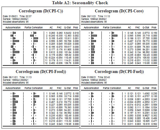
| Table A3: ARIMA Models - Diagnostics | | Models | CPI-C | CPI-Core | CPI-Food | CPI-Fuel | DW
Test Statistic | ARCH
Test for Heterosce-dasticity (P value) | DW
Test Statistic | ARCH
Test for Heterosce-dasticity (P value) | DW
Test Statistic | ARCH
Test for Heterosce-dasticity (P value) | DW
Test Statistic | ARCH
Test for Heterosce-dasticity (P value) | | ARIMA | 2.00 | 0.82 | 1.96 | 0.98 | 2.00 | 0.65 | 1.99 | 0.77 | | SARIMA | 1.98 | 0.77 | 2.02 | 0.96 | 1.97 | 0.51 | 1.99 | 0.77 | | Source: Authors’ estimates. |
| Table A4.1: Roots of Characteristic Polynomial | | Model 1 | Model 2 | | Root | Modulus | Root | Modulus | | 0.64 | 0.64 | 0.59 | 0.59 | | 0.20 | 0.20 | -0.053194 - 0.117008i | 0.128532 | | -0.18 | 0.18 | -0.053194 + 0.117008i | 0.128532 | | 0.10 | 0.10 | 0.02 | 0.02 | Note: No root lies outside the unit circle. VAR satisfies the stability condition.
Source: Authors’ estimates. |
| Table A4.2: VAR Residual Portmanteau Tests for Autocorrelations | | Lag | Model 1 | Model 2 | | Adj Q-Stat | Prob.* | Adj Q-Stat | Prob.* | | 1 | 6.69 | --- | 5.75 | --- | | 2 | 15.19 | 0.51 | 23.88 | 0.09 | | 3 | 37.86 | 0.22 | 46.46 | 0.05 | | 4 | 50.36 | 0.38 | 60.76 | 0.10 | | 5 | 60.49 | 0.60 | 74.88 | 0.17 | | 6 | 83.47 | 0.37 | 91.11 | 0.19 | | 7 | 95.42 | 0.50 | 107.19 | 0.20 | | 8 | 103.01 | 0.72 | 119.11 | 0.31 | | 9 | 116.51 | 0.76 | 132.21 | 0.38 | | 10 | 130.4 | 0.78 | 150.02 | 0.35 | | 11 | 142.67 | 0.83 | 169.03 | 0.30 | | 12 | 158.13 | 0.83 | 180.73 | 0.39 | Note: Null Hypothesis: No residual autocorrelations up to lag h. *Test is valid only for lags larger than the VAR lag order. df is degrees of freedom for (approximate) chi-square distribution; *df and Prob. may not be valid for models with exogenous variables.
Source: Authors’ estimates. |
| Table A5: Percentage Change in Inflation due to a One Percentage Change in Exchange Rate, Output and Interest Rate | | Qtr. | Headline Inflation | Core Inflation | | Exchange Rate Shock | Output Shock | Interest Rate Shock | Exchange Rate Shock | Output Shock | Interest Rate Shock | | 1 | 0.12 | 0.06 | 0.00 | 0.09 | 0.10 | 0.00 | | 2 | 0.09 | 0.22 | -0.15 | 0.04 | 0.18 | -0.16 | | 3 | 0.01 | 0.00 | -0.13 | -0.03 | -0.04 | -0.09 | | 4 | -0.01 | 0.00 | -0.08 | -0.01 | -0.01 | -0.04 | | 5 | -0.01 | 0.00 | -0.05 | -0.01 | 0.00 | -0.03 | | 6 | -0.01 | 0.00 | -0.03 | 0.00 | 0.00 | -0.02 | | 7 | 0.00 | 0.00 | -0.02 | 0.00 | 0.00 | -0.01 | | 8 | 0.00 | 0.00 | -0.01 | 0.00 | 0.00 | -0.01 | | 9 | 0.00 | 0.00 | -0.01 | 0.00 | 0.00 | 0.00 | | 10 | 0.00 | 0.00 | -0.01 | 0.00 | 0.00 | 0.00 | | 11 | 0.00 | 0.00 | 0.00 | 0.00 | 0.00 | 0.00 | | 12 | 0.00 | 0.00 | 0.00 | 0.00 | 0.00 | 0.00 | Note: Exchange rate is represented by INR-USD rate and therefore, an increase (decrease) in exchange rate here implies depreciation (appreciation).
Source: Authors’ estimates. |
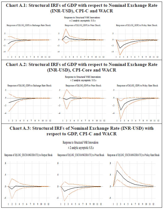 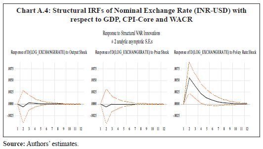
| Table A6: Variance Decomposition of D(Log CPIC) using SVAR Factors | | Qtr. | Headline Inflation | Core Inflation | | Exchange Rate Shock | Output Shock | Own Shock | Interest Rate Shock | Exchange Rate Shock | Output Shock | Own Shock | Interest Rate Shock | | 1 | 3.16 | 0.37 | 96.47 | 0.00 | 1.68 | 1.08 | 97.24 | 0.00 | | 2 | 4.16 | 4.65 | 86.95 | 4.25 | 1.90 | 4.06 | 88.75 | 5.29 | | 3 | 4.02 | 4.48 | 84.57 | 6.93 | 2.01 | 4.16 | 87.06 | 6.76 | | 4 | 3.98 | 4.43 | 83.61 | 7.98 | 2.04 | 4.15 | 86.68 | 7.13 | | 5 | 3.97 | 4.41 | 83.21 | 8.41 | 2.05 | 4.14 | 86.54 | 7.26 | | 6 | 3.97 | 4.40 | 83.05 | 8.59 | 2.05 | 4.14 | 86.50 | 7.31 | | 7 | 3.97 | 4.39 | 82.98 | 8.66 | 2.06 | 4.14 | 86.48 | 7.33 | | 8 | 3.97 | 4.39 | 82.95 | 8.69 | 2.06 | 4.14 | 86.47 | 7.33 | | 9 | 3.97 | 4.39 | 82.94 | 8.70 | 2.06 | 4.14 | 86.47 | 7.33 | | 10 | 3.97 | 4.39 | 82.93 | 8.71 | 2.06 | 4.14 | 86.47 | 7.33 | | 11 | 3.97 | 4.39 | 82.93 | 8.71 | 2.06 | 4.14 | 86.47 | 7.33 | | 12 | 3.97 | 4.39 | 82.93 | 8.71 | 2.06 | 4.14 | 86.47 | 7.34 | | Source: Authors’ estimates. |
| Table A7: NKPC with Survey-based Inflation Expectations (Sample period: 2008-09 to 2017-18Q3) | | | (1) | (2) | | CPI-C (q-o-q change) | CPI-C (q-o-q change) | | 1-year ahead Inflation expectations (y-o-y) | 0.192*** | - | | (0.0497) | | | 3-months ahead Inflation expectations (y-o-y) | - | 0.238*** | | | (0.0546) | | ΔOutput gapt–1 | 0.234** | 0.225** | | (0.0984) | (0.0941) | | ΔOutput gapt–6 | 0.267** | 0.301*** | | (0.111) | (0.108) | | MSP variationt–1 | 0.0398 | 0.0436 | | (0.0556) | (0.0530) | | Rainfall deviationt–2 | 0.0154* | 0.0148* | | (0.00834) | (0.00799) | | ΔExchange ratet–1 | -0.0148 | -0.00943 | | (0.0487) | (0.0460) | | ΔGlobal nonfuel pricet–1 | 0.0585* | 0.0638* | | (0.0335) | (0.0318) | | R2 | 0.627 | 0.659 | | N | 43 | 43 | | Portmanteau test for white noise (Q statistic p-value) | 0.8912 | 0.9042 | Notes: 1. Specifications 1 and 2 include the following quarter dummy variables – 2014q1; 2015q1; 2016q3; and 2018q3. Exchange rate is represented by INR-USD rate and therefore, an increase (decrease) in exchange rate here implies depreciation (appreciation).
2. Inflation expectations are expressed on a y-o-y basis, and therefore, its coefficients need to be multiplied by 4 to make it approximately comparable with the coefficients of trend inflation (which is used as a proxy for inflation expectations) in Table 4.
Standard errors are in the parentheses.
* p < 0.10, ** p < 0.05, *** p < 0.01
Source: Authors’ estimates. |
| Table A8: IV-GMM Estimation – Headline CPIC (q-o-q change in per cent) (Sample period: 1996-97Q1 to 2017-18Q3) | | | (1) | (2) | | CPIC | CPIC | | ΔCPICt+1 | 1.045*** | - | | (6.03) | | | Inflation trendt–1 | - | 1.077*** | | | (5.52) | | ΔCPICt–1 | - | 0.0197 | | | (0.20) | | Output gapt–7 | 0.206*** | 0.191*** | | (3.13) | (2.91) | | ΔOutput gapt–1 | 0.265*** | 0.204*** | | (2.65) | (2.63) | | MSP variationt–1 | -0.0319 | -0.00666 | | (-1.35) | (-0.32) | | ΔExchange ratet–1 | 0.0151 | 0.0307 | | (0.32) | (0.82) | | ΔGlobal nonfuel pricet–1 | 0.0407* | 0.0366* | | (1.70) | (1.74) | | Rainfall deviationt–2 | -0.0113 | -0.00106 | | (-1.50) | (-0.20) | | Uncentred R2 | 0.767 | 0.875 | | Centred R2 | 0.324 | 0.638 | | Adjusted R2 | 0.214 | 0.579 | | Sargan statistic (p-value) | 0.266 | 0.361 | | LM statistic (p-value) | 0.0162 | 0.000 | | N | 80 | 80 | Note: Autocorrelation-adjusted standard errors are used in these regressions. Dummy variables as in the case of earlier models are employed here as well. Exchange rate is represented by INR-USD rate and therefore, an increase (decrease) in exchange rate here implies depreciation (appreciation).
∆CPIt+1 is instrumented with the following variables: Output gapt-6; ∆Output gapt-2; MSP variationt-2; Exchange rate variationt-2; ∆CPIt-1; ∆CPICt-2; and Inflation trendt-2. Inflation trendt-1 is instrumented with Inflation trendt-2; and Inflation trendt–3.
t statistics are in the parentheses.
* p < 0.10, ** p < 0.05, *** p < 0.01
Source: Authors’ estimates. |
| Table A9: IV-GMM Estimation – Core CPI (q-o-q change in per cent) (Sample period: 1996-97Q1 to 2017-18Q3) | | | (1) | (2) | | CPI Core | CPI Core | | ΔCPI Coret+1 | 0.855*** | - | | (5.32) | | | Inflation trendt–1 | - | 0.715*** | | | (3.59) | | ΔCPI Coret–1 | - | -0.00979 | | | (-0.09) | | Output gapt–7 | 0.188*** | 0.153** | | (3.23) | (2.17) | | ΔOutput gapt–1 | 0.375*** | 0.209*** | | (4.03) | (2.75) | | ΔExchange ratet–1 | 0.0484 | 0.0442 | | (1.31) | (1.35) | | ΔIndbasket crudet–1 | 0.0139** | 0.00689 | | (2.30) | (1.25) | | Uncentred R2 | 0.762 | 0.851 | | Centred R2 | 0.206 | 0.501 | | Adjusted R2 | 0.129 | 0.445 | | Sargan statistic (p-value) | 0.245 | 0.547 | | LM statistic (p-value) | 0.00171 | 0.00280 | | N | 80 | 80 | Note: Autocorrelation-adjusted standard errors are used in these regressions. Dummy variables as in the case of earlier models are employed here as well. Exchange rate is represented by INR-USD rate and therefore, an increase (decrease) in exchange rate here implies depreciation (appreciation). ΔCPI Coret+1 is instrumented with the following variables: ΔCPI Coret-1; ΔCPI Coret+1; Crude Oil price variationt-1; and Inflation trendt-2.
Inflation trendt-1 is instrumented with Inflation trendt-2 and Inflation trendt–3.
t statistics are in the parentheses.
* p < 0.10, ** p < 0.05, *** p < 0.01
Source: Authors’ estimates. |
|