Manu Sharma, Arvind Kumar Jha, Anoop K. Suresh and Bikash Maji*

Received on: July 14, 2020
Accepted on: October 14, 2021

The appeal of Monetary Conditions Index either as an operating target or a monetary policy rule has waned over time. Its utility for assessing the monetary policy stance through the lens of alternative channels of monetary policy transmission, however, continues. This paper attempts to construct MCIs for India by approximating four major channels of transmission – interest rate, exchange rate, credit, and asset prices – and examine their suitability to assess the stance of monetary policy as well as the inflation outlook. The weights for these MCIs have been derived using ordinary least squares (OLS) as well as by employing impulse responses of shocks within a structural vector autoregression (SVAR) framework. Empirical findings establish the dominant influence of the interest rate channel in India and support MCIs as useful coincident indicators of monetary policy stance and as a relevant lead indicator of inflation.

JEL Classification: C22, C32, E47, E52, E58

Keywords: Monetary conditions index, interest rate channel, monetary policy, coincident and leading indicator, inflation forecasts

Introduction

The concept of the Monetary Conditions Index (MCI) was introduced by the Bank of Canada (BoC) in 1994, as a weighted average of changes in the domestic short-term interest rate and exchange rate, relative to their respective values in a base period. It was subsequently used in other central banks for specific purposes. MCI measures the degree of easing/tightening in monetary conditions, and thus, reflects the overall stance (expansionary/ contractionary) of monetary policy for a given period (Freedman, 1994, 1995). Apart from its role as an indicator of monetary stance, the literature suggests that MCI can be used as a monetary policy operating target (Freedman, 1994) or even as a policy rule (Ball, 1999). For its use as an operating target of monetary policy, a target level of MCI needs to be identified in accordance with the policy objectives, and monetary policy operations conducted to make the actual level of MCI as close as possible to the target level. On the other hand, the use of MCI as a policy rule is close to exchange rate targeting since it requires interest rate to be set in such a way that it ensures alignment with the changes in the exchange rate (Batini and Turnbull, 2002). The use of MCI as an operating target for monetary policy or as policy rule has serious caveats (Freedman, 1994) that range from inability to identify shocks to the economy in general to the volatile nature of exchange rates in particular. As a result, while no central bank uses MCI as a policy rule, the Reserve Bank of New Zealand discontinued using MCI as a monetary policy target in the wake of the MCI led monetary policy uncertainties in New Zealand (Svensson, 2001; Mishkin and Schmidt-Hebbel, 2001). On the other hand, since MCI also indicates the resultant effect of monetary transmission channels on aggregate demand and inflation, its potential to act as a leading indicator for short to the medium-term impact of monetary policy on the economy has come to the forefront (Goodhart and Hofmann, 2001; Guillaumin and Vallet, 2017; Horry et al., 2018).

In India, against the backdrop of ongoing financial deregulation/ innovations, a vibrant banking sector and increasing integration among the financial markets; multiple channels of monetary policy transmission play a role in influencing the overall monetary conditions. Therefore, this paper attempts to construct MCI in a ‘broad’ way for India covering the four major monetary policy transmission channels viz., interest rate, exchange rate, credit, and asset prices¹ (as a weighted average of four real variables - short-term interest rate, exchange rate, bank credit and BSE Sensex - representing the four channels). The weights are expected to provide a gauge on the relative importance of different channels in monetary policy transmission. This study not only attempts to address the much-discussed challenges that have been put forward in the literature relating to the econometric techniques employed in deriving weights of MCI² but also briefly covers the fact that the very construct of the index is equally important. It further analyses the ability of the MCI to capture the monetary policy stance of the Reserve Bank as well as its potential in predicting Consumer Price Index (CPI) inflation in India.

The structure of the rest of this paper is as follows. Section II describes the four channels of monetary policy from the standpoint of their specific dynamics in relation to the ultimate goal variables. Section III specifies the theoretical construct that underpins MCI. Section IV presents a brief literature survey covering empirical findings of available research on the subject and international experiences. Section V describes the data and methodology employed for deriving the weights of different variables in the construction of MCI for India. Section VI presents the results and empirical analysis, validating the utility of MCI in the Indian context. Section VII provides concluding observations.

Section II
Monetary Policy Transmission Channels – A Foundation for MCI

The choice of an intermediate target of monetary policy depends upon the information content it may have to forecast the goal variable. At times, using the intermediate target is equivalent to targeting the forecast of the goal variable (Bernanke and Mishkin, 1997). During the monetary targeting regime in India, with Cash Reserve Ratio (CRR) as a major instrument and Reserve Money as an operating target, the choice of monetary aggregates (Money Supply) as intermediate target seemed justified due to the ability of the operating target to directly influence the intermediate target which itself had a stable relationship with prices and output (Mohanty, 2011). In the Multiple Indicators/Augmented Multiple Indicators Approach, a host of forward looking macro-economic indicators and a panel of times series models were used to shape an outlook of growth and inflation (Mohanty, 2011). Money supply projections still served as an important information variable. However, owing to growing instability in the relationship between the money supply and the ultimate goal variables (inflation and growth) as well as the difficulties faced by the Reserve Bank in controlling the money supply through CRR and Statutory Liquidity Ratio (SLR) in the 1990s, its position as an intermediate target became untenable. Under flexible inflation targeting (FIT) framework with weighted average overnight call money rate (WACR)³ as an operating target, although the Expert Committee (RBI, 2014) did not explicitly mention the intermediate target, it is argued that ‘inflation forecast’ acts as the intermediate target in practice⁴.

The stance of the monetary policy affects the intermediate target and further the final target through monetary policy transmission channels. The literature and also the Expert Committee (RBI, 2014) identifies four such major channels:

1. Interest rate channel: Expansionary (contractionary) monetary policy stance → decrease (increase) in interest rate → decrease (increase) in the cost of capital → increase (decrease) in investment → increase (decrease) in aggregate demand → prices rise (fall)⁵

2. Exchange rate channel: Expansionary (contractionary) monetary policy stance → depreciation (appreciation) in domestic currency → net exports rise (fall) → increase (decrease) in aggregate demand → prices rise (fall)⁶

3. Credit channel: Expansionary (contractionary) monetary policy stance → fall (rise) in the interest rate and expansion (contraction) in loanable funds → decrease (increase) in the cost of funds and bank lending rates → demand for bank credit rise (fall) → increase (decrease) in aggregate demand → prices rise (fall)⁷

4. Asset price channel: Expansionary (contractionary) monetary policy stance → cheaper (dearer) borrowing costs → higher (lower) asset prices → higher (lower) household/corporate wealth effect and cash flows→ increase (decrease) in aggregate demand → prices rise (fall)⁸

It is indeed difficult to gauge the individual impact of these monetary policy transmission channels since they tend to co-exist with different degrees of effectiveness, often interact with each other, thus, supplementing/offsetting each other (Acharya, 2017) through a host of variables. They simultaneously impact the intermediate target (inflation forecast under FIT) which itself gives a proximate view of the course of policy goal variables (inflation and economic growth), in fulfilment of the overall policy goal of price stability and economic growth. The lags at which monetary policy impacts final demand and inflation differs depending upon the stage of the business cycle, fiscal position, liquidity and financial conditions and the health of the financial system. In the case of India, on average, the monetary policy action takes around 2 to 3 quarters to show its impact on output and 3 to 4 quarters in impacting inflation and the impact persists for 8 to 12 quarters (Acharya, 2017). The interest rate channel has been highlighted in the empirical research in India as the most important channel for monetary policy transmission (RBI, 2014).

Hence, within the overall monetary policy framework, although studying the movement of the operating target (WACR) may be enough to draw a perspective of monetary policy stance⁹, to study the implications of this stance on key policy goal variables like inflation and growth, the multiple monetary policy transmission channels, and the related variables (with different lags at which they impact the policy goal variables) should be factored in. This understanding is of utmost importance for constructing MCI, which, in this study, is envisaged as a coincident indicator of monetary policy stance as well as a leading indicator of inflation.

Section III
Literature Review and International Experience

The Canadian monetary policy, over time, has been one that has been subjected to drastic changes. In the pre-1990s, the focus of the Canadian monetary policy was the attainment of intermediate targets. However, since the early 1990s, the BoC has adopted inflation targeting alongside MCI as an operational target. The central banks of New Zealand, Sweden, Norway, and European Monetary Union had also used MCI, customised to their requirements. The compilation of MCIs periodically is also undertaken by several international organisations such as the IMF, OECD, and commercial banks for cross country assessment of monetary policy and their monetary conditions.

Kesriyeli and Kocaker (1999) constructed MCI for Turkey utilising monthly data on prices, interest rates and exchange rate covering the period 1988-1997, wherein exchange rate turned out to be a significant factor determining adjustments in prices in Turkey. Batini and Turnbull (2000) undertook a survey of MCIs constructed for the UK by various multinational institutions. Through a macro-econometric simulator model (covering 15 years from 1984 to 1999), they constructed another MCI for the UK, paying adequate attention to overcoming several drawbacks of the exiting MCIs. Kodra (2011) constructed the MCI of Albania by using the ordinary least squares (OLS) estimator and data between 1998 and 2008. The author undertook an assessment of exchange rate and interest rate in real terms and found that a rise in the real exchange rate by 3.8 could be equivalent to a rise in real interest rate by one per cent.

Siklar and Dogan (2015) assessed the effect of changes in exchange rate and interest rate on Turkey’s monetary policy by using MCI. The estimation of MCI using Kalman Filter is a special feature of this paper (i.e., the time-variant component vis-à-vis the constant weighted MCI in several other papers). The study concludes that movements in price level could lead to movement in both exchange rate as well as interest rates. In line with the findings of other major studies on MCI, it concludes that the interest rate channel creates a profound impact on the economy (vis-à-vis exchange rate channel). Jovic et al., (2018) undertook the construction of MCI for Bosnia and Herzegovina (BH) utilising a multiple linear regression approach. The study brought out two important findings. First, in the post-2008 crisis period, there has been an improvement in monetary conditions in BH. Second, the interest rate channel when compared with the exchange rate channel does not turn out to be very dominant.

Apart from these studies at the cross-country level, there have been few studies that attempted constructing an MCI for India. In one of the pioneer works in India during the monetary targeting regime, Patra and Pattanaik (1998) attempted to develop indices of exchange market pressure, intervention activity and monetary conditions using a sample period of April 1990 to March 1998. Kannan et al., (2006) constructed an MCI based on both the exchange rate and interest rate channels as well as incorporating an additional component (i.e., credit). According to this study, interest rate turns out to be the most significant variable that determines India’s monetary settings. Bhattacharya and Ray (2007) introduced a measure of the stance of India’s monetary policy covering the period from 1973 to 1998. Utilising an autoregressive approach, the authors connected the constructed MCI with prices as well as output, and find the monetary policy in India to be more effective in combating price rise rather than catalysing output expansion. Samantaraya (2009) introduced an index for evaluating the effect of monetary policy on key macroeconomic variables.

Section IV
Theory and Construct

The exercise for constructing MCI can be broadly divided in four consecutive stages with one complementing the other – (1) Identification of the monetary policy transmission channels and the respective relevant representative variables; (2) Finalising the Construct of MCI equation; (3) Selection of the target variable (defined subsequently) for deriving weights of MCI; and (4) Estimating the weights using econometric models to generate the index. These aspects are discussed in detail in this section.

(1) Identification of the monetary policy transmission channels and the representative variables

MCI has conventionally been defined as a weighted average of changes in the short-term interest rate and changes in the exchange rate for an open economy. However, off-late many versions of MCI cover multiple monetary policy transmission channels¹⁰. In this study, we have accounted for the four channels (Acharya, 2017 and RBI, 2014) which are already discussed in Section II. Their representative variables – real WACR, real effective exchange rate (REER) index, real bank credit and real stock price index – are described in Appendix I.

(2) Finalising the construct of MCI

In most of the studies related to MCI, much of the attention is given to the econometric methods employed to estimate the weights of the constituent variables, while the construct of MCI itself often takes a backstage. As a result, the final understanding of the construct and the variables employed is left to the imagination of readers. The original structure of MCI as provided by Freedman (1994) is:

where, r_t is the real short-term interest rate and e_t is the real effective exchange rate index (where a rise represents an appreciation) at time t, while r_b and e_b represent the values of corresponding variables in a given base period b. α₁ and α₂ are the weights assigned to the two variables, respectively.

It is important to note that since interest rates are presented in percentage terms, the exchange rate is also taken as per cent change i.e., the units of measurement of both interest rates as well as exchange rate are kept the same. Somewhat similar is the approach adopted by Batini and Turnbull (2002), who create a ‘Dynamic MCI’ wherein logarithm values of real effective exchange rate are used, and interest rates are presented as fractions by dividing interest rate data by 100. Toroj (2008) uses a similar construct, but instead of presenting interest rate as a fraction, he divides interest rate and exchange rate variables (logarithm values) by their respective standard deviations across the sample period. In all these approaches, the synthesis imparts uniformity of scale/measurement to the weighed impact of different variables (representing different monetary transmission channels) on MCI.

Another set of studies, e.g., Hataiseree (1998) and Kannan et al. (2006)¹¹ alternatively present MCI as:

where, the real exchange rate/effective exchange rate is expressed in the logarithm values while no transformation is reported for interest rates. This construct makes MCI closely reflect the short-term interest rate path, which gets partly complemented/offset by the movement in the exchange rate, and thus, quite appealing as a reflection of the monetary stance of the central bank.

Another construct proposes de-trended MCI by doing away with the concept of ‘base period’. This non-conventional approach brings MCI closer to the much-discussed Financial Conditions Index¹² (Goodhart and Hofmann, 2001; Khundrakpam, 2017):

In the present study, we have broadened the concept of MCI by including economic/financial variables representing the four major transmission channels thus endorsing its usefulness in gauging the impact of monetary policy instruments on financial variable as a result of monetary policy transmission. However, for maintaining the ability of MCI to act as a coincident indicator of the stance of monetary policy, the basic approach as indicated in equation 2 has been adopted. This has been augmented with the de-trending method as suggested in equation 3. Accordingly, for this study, MCI has been computed using four real variables i.e., real short-term interest rate, real effective exchange rate (REER) index, real bank credit and real stock price index, such that¹³: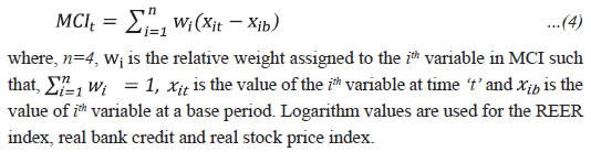

Generally, the variables in MCI are set in relation to their respective levels in a base period. Accordingly, two MCIs are constructed using this base period approach by taking the start of the sample period as 1996-97:Q1. This way, MCI starts at 0 for 1996-97:Q1 and the subsequent tightening or loosening of the monetary stance can be viewed in relation to the base period. While it’s important to note that the numerical value of MCI at any time ‘t’ is meaningless, it’s the movement in MCI vis-a-vis the base period that reflects the monetary stance. An increase in MCI depicts expansionary monetary policies and vice versa. However, when the base period is used, the analysis of MCI movement becomes bi-dimensional i.e., in relation to the base period as well as in relation to the lagged value. In the study, we follow a de-trending approach for the construction of a third MCI, wherein variable values are set in relation to long-run trend or equilibrium such that: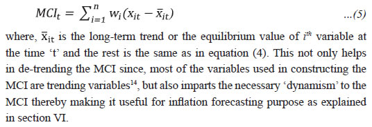

(3) Selection of the target variable for deriving weights of MCI

The target variable for MCI is the variable which the monetary conditions try to influence. The choice of target variable for constructing MCI coincides with the choice of the final target variable for monetary policy framework since MCI incorporates the impact of different transmission channels (although at different degrees) that finally influence the policy goal variables in fulfilment of the policy goal. Thus, aggregate demand and inflation¹⁵ automatically emerge as the preferred choices. Under monetary targeting, the sensitivity of money demand to changes in the exchange rate and interest rate provides the relevant target for MCI (Patra & Pattanaik, 1998). Under the inflation targeting, the sensitivity of aggregate demand and/or inflation to changes in the interest rate and exchange rate could provide more relevant targets for MCI. In this study, real GDP growth has been used as the target variable for MCI, while Consumer Price Index-Combined (CPI-C) based inflation has also been considered separately as a target. The choice of CPI-C based inflation is commensurate with the present monetary policy framework and usage of real GDP growth instead of the output gap is justified because the dynamics of an evolving/emerging economy make it difficult to estimate the economy’s optimal level of operating efficiency and thus, the potential output, which is required to generate the final output gap.

(4) Estimating the weights using econometric models to build an index

Different methods can be used for estimating MCI weights (Batini and Turnbull, 2002; Guillaumin and Vallet, 2017):

1. OLS equation-based weights: The weights of MCI are derived from the coefficients of a regression equation estimating either aggregate demand or inflation. This is the most common method owing to its simplicity. In the case of India, Kannan et al., 2006 estimated MCI using this technique.

2. Trade share-based weights¹⁶: The weight for the exchange rate is obtained from the long-run exports-to-GDP ratio. The weight for the interest rate is one minus the weight for the exchange rate.

3. VAR impulse response functions-based weights: The weights are obtained using the impulse responses of the target variable to the shocks in endogenous variables in a reduced form Vector Auto Regression (VAR) framework (Eika et al., 1996). Either cumulative (as is the practice at Goldman Sachs for the UK) or average (Goodhart and Hofmann, 2001) of the impulse responses can be used.

4. Large-scale simulations based macro-econometric models: These include certain complex and exhaustive models used by the central banks/institutions which take many variables at a time into account for modelling the overall structure of the economy (Mayes and Viren, 2001; Costa, 2000).¹⁷

In general, the literature is flourished with critics of the econometric methods employed for deriving the weights of MCI (Eika et al., 1996; Ericsson et al., 1998; Stevens, 1998). Some downsides most commonly cited critics are model dependence, lack of dynamism in the model specification, parameter inconstancy, non-exogeneity of regressors, cointegration among non-stationary variables and the choice of variables. This study attempts to minimise these issues in a variety of ways. The issue of model dependence, like any other econometric exercise, is valid in this case too. Since weights obtained depend upon the model specification, adequate attention has been given to ensure that the model is suitably specified keeping in view the overall dynamics of monetary policy transmission. Further, to analyse the impact of the choice of model, both- single equation models, as well as impulse responses derived from a structural VAR (SVAR) model have been used, to estimate the weights for MCI and compare them. Variables are found to be stationary and so chances of co-integration are ruled out. Structural breaks have been tested for and dummy variables have been included wherever required, along with necessary stability tests to ensure the model stability. The non-exogeneity issue does seem to apply to this study due to forward-looking nature of the variables, potentially leading to problems such as simultaneity bias. However, a central bank responds to macroeconomic changes by taking a monetary stance which in turn impacts various economic variables, and hence, it would be naive to consider monetary conditions as totally exogenous. Moreover, monetary transmission works by impacting its target variable (aggregate demand or inflation) with lags and dynamic interaction of endogenous/ exogenous variables, taking care of simultaneity to some extent. Nonetheless, we attempt to address these problems by additionally specifying a SVAR model, which identifies a system of equations for endogenous variables interacting with each other (as against a single equation with a built-in assumption of ceteris paribus) and identifies structural shocks for impulse responses, imposing required restrictions as per the economic theory, to confine the contemporaneous relationships.

The theory suggests that the decrease in real interest rates and REER index, and an increase in real credit and real stock price index reflects an expansionary stance and hence increasing the MCI and vice versa. Thus, it is expected that in the MCI, the weights of real short-term interest rate and REER are negative while those for real credit and real stock price index are positive.

Section V
Data and Methodology

The data used for empirical analyses are sourced from the Database on Indian Economy (DBIE) and Reserve Bank of India website (www.rbi.org.in), for the period 1996-97:Q1 to 2019-20:Q3. The choice of this period is guided by the availability of quarterly GDP at Market Prices (Constant Prices) Data Series (Base 2011-12). Further details about data are furnished in Appendix I.

Two methodologies i.e., reduced form estimates of coefficients in an OLS model [both Aggregate Demand (AD) and Phillips Curve (PC) equation] and impulse response functions in a SVAR model, have been adopted for estimating the weights for three alternative MCIs: MCI_AD, MCI_PC and MCI_SVAR. All the variables are Stationary at levels (Appendix II).

Ordinary Least Square Model

MCI_AD: The weights have been derived by estimating the generalised backward looking aggregate demand equation, which is represented as:

where gdpg is the y-o-y growth rate of real GDP, wacr is the real weighted average call rate, reertg is the y-o-y growth rate of trade weight-based real effective exchange rate (36 currency based), bcrg is the y-o-y growth rate of real total bank credit, snsxr is the real y-o-y sensex returns, ϵ_t is the residual term and α₁ is a constant signifying natural rate of real GDP growth. t refers to the contemporaneous time specification while i, j, k, l, and m are lags for the specific variable.

Inclusion of long-term interest rates in equation (6) in many studies (Hyder and Khan, 2006; Deutsche Bundesbank, 1999; Mayes and Viren, 2001) presents another school of thought where long term interest rates are equally relevant for estimating aggregate demand conditions. Although, there is existing literature in relation to long term real interest rates in India (Behera et al., 2015), in accordance with the limitation of such long term interest rates (Wahi and Kapur, 2018) and also in line with the views of Goodhart and Hofmann (2001), we believe that such real long term interest rates are difficult to get (owing to challenges in obtaining long-term inflation expectations/long term inflation measures matching the maturity of the bond underlying the long-term yield).

No significant structural breaks were found in the data. A dummy variable named “dumgfc” is included to account for the impact of the global financial crisis that dampened aggregate demand in India during 2008:Q2 - 2008:Q4. The dynamics of the model had been specified by incorporating only the most significant lags of the dependent variable as well as independent variables.

MCI_PC: The weights have been derived by estimating a backward-looking Phillips curve equation which can be derived on the lines of Fisher et al., (1997), using the following relationship between the rate of inflation and output gap:

where, ∆p is the rate of inflation, ∆p_-t is the rate of inflation witnessed in the past, ∆p^e is the inflation expectation, ŷ is the output gap and λ is a measure of persistence. The equation summarises the role of the economy as well as the economic agents in setting up the prices. The economic agents indeed respond to the past value of inflation as well as its expectation which can be given as:

where, ṕ is the central bank’s inflation target and μ measures the credibility of the central bank’s inflation target. Hence, the inflation expectation can be thought of as a weighted average of the past inflation and the central bank’s inflation target.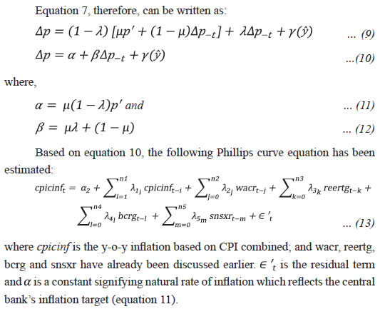

The independent variables of this regression, including real WACR, REER growth, real bank credit growth and real stock market returns, are the determinants of aggregate demand (equation 6). Since the output gap more or less represents the cyclical component of this aggregate demand, the independent variables can be considered as a part of the broad economic frame that determines the output gap¹⁸. No significant structural breaks were found in the data, barring a few instances of volatilities including the peaks in inflation on account of implementation of 5th and 6th Central Government Pay Commissions. However, upon entering a dummy variable to account for these in the equation, the same was found to be insignificant and hence excluded from estimation. The dynamics of the model have been specified by incorporating only the most significant lags of the dependent variable as well as independent variables.

Structural Vector Autoregression (SVAR) model

MCI_SVAR: The SVAR model is used instead of the standard reduced-form VAR model because the former provides explicit behavioural interpretations of all parameters, and thus, reflects the well-defined dynamics (in terms of the economic structure) among the variables considered in the model.

Within a SVAR framework, a reduced form VAR model has been specified as follows: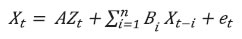

where, X is the vector of six endogenous variables – cpiinf, wacr, reertgap, crgap, snsxgap and gdpgap. wacr represents short term interest rates expressed as per cent; cpcinf is the four-quarter lag of log difference in seasonally adjusted CPI-C (y-o-y) inflation; and reertgap, crgap, snsxgap and gdpgap represent the ratio of the cyclical to trend component of the logarithm value of REER, real bank credit, real sensex and real GDP (seasonal adjustment is done wherever needed), respectively.¹⁹ The cyclical and trend component have been derived using HP filter with a lambda value of 1600 owing to the use of quarterly data. This gap approach presents a departure from the commonly used growth approach and appears more appealing in a context where the aim is to measure the impact of deviation of variables from their potential levels. This novel approach finds support in the existing literature too (Goodhart and Hofmann, 2001; Guillaumin and Vallet, 2017).

Z_t contains exogenous variables including intercept and two dummy variables to account for outliers in the residuals; e_t is the vector of error terms/ forecast errors of the VAR process and n is the number of lags included. Based on AIC, 5 is chosen to be the lag length (Appendix V).

B₁ to B_n are n x n coefficient matrices of lagged endogenous variables and A is the matrix of coefficients of exogenous variables.

Moving further, SVAR has been estimated by decomposing residuals into structural shocks by ascertaining the contemporaneous relationship between standard reduced form and structural innovations. For this matrix B needs to be calculated, such that:

where e_t is the vector of estimated residuals/forecast errors of the standard VAR system and ϵ_t is the vector of structural shocks/innovations.

Having assumed that structural shocks are orthogonal²⁰ to each other, matrix C contains the contemporaneous influence of structural disturbances on endogenous variables, such that: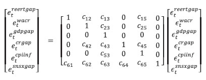

The c_ij element of the structural matrix is the magnitude by which the j^th structural shock affects the i^th variable simultaneously. In a broad manner, the C matrix represents that real GDP responds rather slowly to shocks in inflation, real interest rate, real effective exchange rate, real bank credit and real stock returns. Response of inflation is slow to shocks in real interest rate, real effective exchange rate, real bank credit and real stock returns but inflation reacts immediately to shocks in real GDP. Real interest rates react instantaneously to shocks in real GDP and inflation (the construct of Taylor’s Rule) while the same is not true for the shocks on real bank credit, real effective exchange rate and real stock returns. Moreover, real bank credit and real effective exchange rate respond immediately to shocks in real GDP, inflation, and real interest rates. On the other hand, stock returns that reflect market sentiments respond contemporaneously to shocks in all the given variables.

For identification purposes²¹, the point zero restriction approach (Vonnak, 2005; Khundrakpam, 2012) has been used, which restricts some elements of matrix C to zero. This strategy has the advantage that a structure of contemporaneous impacts can be translated to delayed reaction (Khundrakpam, 2012).

Section VI
Results

The result of the OLS regression for aggregate demand equation is summarised in Table 1.

As evident, the signs of the coefficients of independent variables are in sync with the economic theory. An increase in interest rates and a rise in the effective exchange rate (leading to domestic currency appreciation), ceteris paribus, dampens aggregate demand while the reverse is true for an increase in bank credit and stock returns during the period of the study.

The results for diagnostic tests and stability tests for the model are summarised in Appendix III. They rule out the presence of autocorrelation in the residuals as well as heteroskedasticity. Moreover, they confirm that the residuals are normally distributed. Additionally, parameter stability is established in CUSUM and CUSUM of squares test. The estimated coefficients in aggregate demand equations suggest the weights of MCI_AD for real WACR, REER index, real bank credit and real sensex to be -0.47 and -0.32, 0.16 and 0.05, respectively. Accordingly, MCI_AD has been created following the classical approach as mentioned in equation 4 i.e., on a base period that has been fixed at the beginning of the data sample i.e., 1996Q1.

The result of the OLS regression for the Phillips Curve equation are summarised in Table 2.

The signs of the coefficients of independent variables in Table 2 are as expected. An increase in interest rates and effective exchange rate, ceteris paribus reduces inflation while the reverse is true for bank credit and stock returns during the period of the study. Except for REER, all other variables are significant at a 5 per cent level of significance. R squared and adjusted R squared measures have also improved. This marks an improvement over the previous model.

Appendix IV summarises the results for diagnostic checks and model stability tests which confirm the absence of heteroskedasticity and autocorrelation in the residuals and that the residuals are normally distributed. Additionally, parameter stability is established by CUSUM and CUSUM of squares tests. The estimated coefficients in the aggregate demand equation suggest the weights of MCI_PC for real WACR, REER index, real bank credit and real sensex to be -0.58 and -0.17, 0.20 and 0.05, respectively. Accordingly, MCI_PC has been created following the classical method as given in equation 5 i.e., on a base period which has been fixed at the beginning of the data sample i.e., 1996-97:Q1.

For the SVAR system, the LR test for over-identification cannot be rejected at 5 per cent significance level, thus validating the imposed restrictions. Moreover, the SVAR is found to be stable since the inverse roots of the characteristic polynomial lie within the unit circle (Appendix V), which can also be viewed as a general fallout of all the endogenous variables being stationary. Appendix V further summarises the result of other diagnostic tests which confirm that VAR residuals are normally distributed and do not suffer from serial correlation and heteroskedasticity. For calculating the weights of MCI_SVAR, impulse response functions are obtained for responses of cpiinf to one standard deviation positive structural innovations/ shocks in wacr, reertgap, crgap and snsxgap in a two standard error band over a period of 12 quarters (Appendix V). The direction of responses is mostly as expected. A positive shock in wacr decreases inflation and a positive shock in crgap and snsxgap increases cpiinf. These impulse responses are statistically significant at around the period of peak impact. The response of cpiinf to a positive shock in reertgap is not highly significant and is also mixed in terms of direction. The average²² of the numerical value of the response of inflation to one standard deviation positive shock to each variable over 12 quarters suggests the weights of MCI_SVAR for real WACR, REER index, real bank credit and real sensex to be -0.35 and -0.14, 0.35 and 0.16, respectively. Accordingly, MCI_SVAR has been created. However, this MCI follows the detrending approach as mentioned in equation 5 i.e., without fixing a base period, as discussed earlier.

Table 3 summarises the obtained weights of real WACR, REER, real bank credit and real sensex using the above-mentioned three methods i.e., aggregate demand equation, Phillips Curve equation and SVAR.

The weights for the variables (representing the respective channels) have been derived by normalising the coefficients/impulse responses of the concerned variables such that they add up to one in the case of each MCI. Hence, their magnitude represents the relative ability of the respective channel of transmission in influencing MCI and thus, the overall monetary conditions. Irrespective of the model applied, the direction/sign of the estimated weights (negative/positive) are in sync with the economic theory validating the robustness. A positive sign indicates an increase in MCI reflecting easing of the monetary conditions and vice versa. Further, parameter stability is established, as already discussed in this section, thus ensuring the stability of weights. Further, this is in direct consensus with a plethora of available literature which suggests that credit exerts a pro-cyclical impact on aggregate demand (Kannan et al., 2006; Bernanke and Gertler, 1995). This is all the more important for a banking dominated economy like India where bank credit movements are often tracked to assess the effectiveness of the monetary policy. Moreover, the impact of the stock market on aggregate demand is well established (Blanchard, 1981; Khundrakpam et al., 2017), operating through wealth effect and expectations. Although there is no denying the fact that the credit channel assumes importance, the interest rate channel dominates with the highest weight, justifying its suitability as the instrument of monetary policy.

MCI and the Monetary Stance

The obtained MCIs are presented in Chart 1. As discussed earlier, rather than the exact values of MCIs at any point of time, it is the direction of movement which is relevant. All the three MCIs exhibit broadly similar patterns with the major difference that MCI_SVAR lacks a specific long-term trend as per its construct. The MCIs provide some useful information about various phases of monetary easing/tightening.

The ‘monetary targeting approach’²³ was replaced in India by the ‘multiple indicator approach’²⁴ during 1998. The period from 1997-1999 witnessed some massive upheavals including economic sanctions over India due to the Nuclear testing programme, followed by the Asian Financial Crisis, Russian debt crisis and the Long-Term Capital Management (LTCM) debacle. In response, despite inflationary pressures, an expansionary monetary stance was adopted initially to support the growth momentum and maintain comfortable liquidity conditions, anticipating the international liquidity and export restrictions, which nevertheless shifted to a tightening mode in the wake of a price spiral, depreciating currency and capital outflows requiring the interventions in forex markets. This was shortly followed by an expansionary stance during the early 2000s, amidst benign inflation, in view of the economy experiencing a slowdown in growth due to domestic reasons (weakened demand due to deficient monsoons in 2000) and external disruptions (due to the Dot com bubble which impacted stocks of various international IT firms, there was a need to insulate Indian IT firms from the said shock).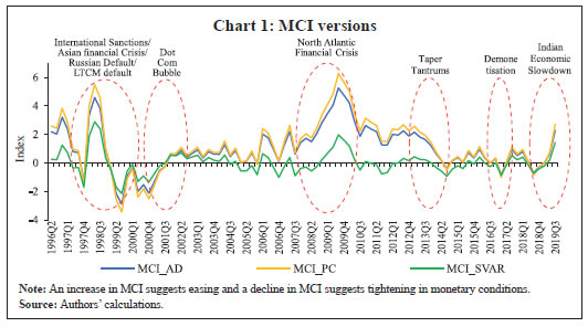

The period from 2003-2008 witnessed the firming of economic growth (Chart 2) and concomitant expansion in credit demand. Moreover, aggregate demand pressures overheated the economy following high capital inflows which led to surplus liquidity conditions fuelling credit supply and asset prices soared.

On the inflation front, although the implementation of fiscal rules in 2004-05 and real appreciation in exchange rates due to steady capital inflows eased inflationary pressures till 2005-06. An upswing in the general commodity prices and the lagged pass-through of an upsurge in global crude prices to administered prices in India pulled up inflation afterwards. In response, the repo rate was raised to 9 per cent by 2008-09, having witnessed a cumulative increase of nearly 300 basis points from 2005-06 to 2008-09. However, in real terms, it witnessed a steep fall. As a result, a range of monetary policy actions were simultaneously undertaken, including increment in cash reserve requirement (CRR) to the tune of 400 bps (from 5 per cent to 9 per cent during 2004-08) and introduction of a market stabilisation scheme to absorb surplus domestic liquidity and sterilise the impact of intervention operations carried out in the wake of unparalleled capital inflows. Implementation of stricter risk weights and other provisioning norms to moderate the credit boom, were some of the additional macro-prudential measures undertaken to control asset price inflation. Thus, the whole period was marked by a cautious and prolonged tightening in the monetary policy stance. MCI_SVAR reflects this in a slightly better way.

The following period marked the advent of the much-debated North Atlantic Financial Crisis of 2007-08, which escalated into the so-called ‘Global Financial Crisis’. Although owing to its strong economic fundamentals and also limited exposure to global mortgage and derivative markets, India remained insulated from the crisis at large, however, transient disruptions in short-term inter-bank markets and a temporary but sharp slump in the economic activities was witnessed due to contraction in external demand and the squeezed bank lending. This was met with expansionary monetary as well as fiscal measures. Macro-prudential measures (including easing of risk weights and provisioning norms for standard assets, focused primarily on real estate and NBFC sector) were undertaken and the economy witnessed a sharp growth rebound. Inflation as reflected by CPI, on the other hand, remained high through the crisis period till 2013 owing to persistent food and fuel inflation. While monsoon shocks of 2009 fed to supply-side pressures, fiscal interventions through a substantial increase in minimum support prices (MSP) and a considerable increase in the coverage under the MGNREGA aided the demand-side pressures. Thus, apart from normalising the crisis led expansionary monetary policy, tightening monetary policy measures were further undertaken attuned to persisting inflation and fiscal expansion till the beginning of 2012. Subsequently, in the wake of the growth concerns and stabilising inflation, monetary policy easing was pursued during 2012 and the first half of 2013.

The global impact of the crisis culminated in the much-discussed ‘taper tantrum’ of 2013. The Reserve Bank stepped in with stabilising measures to curb excessive volatility in the foreign exchange market. The persistently high inflation during the post-crisis period, however, exposed the fault lines in macro-financial stability and paved the way for a review of the monetary policy framework, leading to the Reserve Bank endorsing the ‘glide path’ of CPI inflation in the beginning of 2014 and the subsequent adoption of FIT in 2016.

Meanwhile, falling commodity prices including crude oil prices, softening food inflation and more or less steady exchange rates led to a broad-based decline in inflation in accordance with the prescribed ‘glide path’. Accordingly, an expansionary monetary policy stance was adopted till April 2016 to support growth. Finally, in May 2016, the Reserve Bank of India Act, 1934 was amended, enabling the adoption of FIT with price stability as the primary objective and CPI as the nominal anchor for monetary policy. In the ensuing period, monetary policy response balanced the need of moderating inflation and inflationary expectations while supporting growth, steering the economy through some major events including demonetisation until 2018, when the economic slowdown hit the Indian economy and the monetary stance became accommodative with a lower interest regime kicking in.

A historical analysis of the past economic events in a phase-wise manner endorses the role of MCI as a coincident indicator of monetary stance. A multivariate VAR has been estimated with MCI’s, inflation, and real GDP growth. Lag order has been selected based on recommended lag order selection criteria (Hannah Quinn lag selection criteria). The results suggest that inflation and real GDP growth Granger causes MCIs at 1 per cent to 5 per cent significance level (Appendix VI). This indicates that the developments on the front of the economic growth and inflation are feeding back on the course of monetary policy actions by the Reserve Bank in the form of the monetary stance which further gets reflected in the movement of MCIs. This endorses the ability of MCIs to reflect the monetary stance of the Reserve Bank in response to the two policy goal variables in light of the primary objective of monetary policy under the FIT framework i.e., to maintain price stability while keeping in mind the objective of growth.

MCI and Inflation Prediction

In view of the forward-looking nature of monetary policy; particularly under FIT framework, and the importance of inflation forecasts as the intermediate target; the MCI could be useful as a leading indicator of inflation (Chart 3 plots MCIs along with CPI inflation).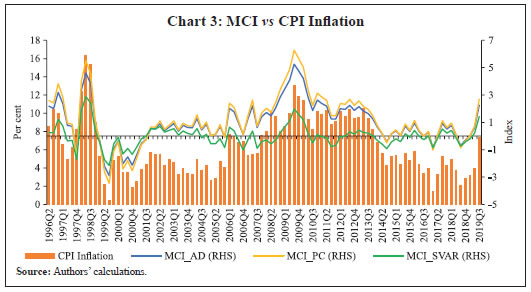

In the multivariate VAR set up mentioned before, the results (Appendix VI) suggest that only MCI_SVAR exhibits a bi-directional causality with inflation i.e., inflation Granger causes MCI_SVAR at 5 per cent significance level and MCI_SVAR Granger causes inflation at 1 per cent significance level. This shows that the lagged values of MCI_SVAR may contain information about future inflation. To further support this finding, as also to address the much-discussed reservation that the Granger causality proposed by Granger (1969) may suffer from specification bias and spurious regression (in addition to a probable nonstandard distribution in the presence of unit roots and structural breaks), we further test the TYDL Granger causality (Toda and Yamamoto, 1995; Dolado and Lutkepohl, 1996) based on augmented VAR. The results (Appendix VII) endorse the bi-directional causality between MCI_SVAR and inflation at 1 per cent significance level.

Moreover, the impulse response functions (including accumulated ones), identified based on Cholesky as well as Generalised factorisation on a bivariate VAR set up including inflation and MCI_SVAR, also indicate that shock in MCI_SVAR generates strong and significant impulse responses of inflation.

To summarise, if the information contained in the lagged values of inflation can be controlled, the lagged values of the MCI_SVAR can predict current CPI inflation and thus MCI_SVAR can be used as a leading indicator/ high-frequency indicator for forecasting CPI inflation.

Results of Forecasting Performance of MCI_SVAR

We attempt an inflation forecasting exercise (out of sample forecast) to evaluate the predictive power of MCI_SVAR for future inflation by estimating the following equations: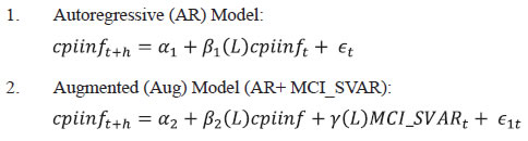

where h is the horizon of forecast; MCI_SVAR is the estimated monetary conditions index based on SVAR and β₁(L), β₂(L) and γ(L) are polynomials in the lag operator L. A rolling window of 10 lags has been taken for different values of h, where h ranges from 1 to 3 quarters i.e., generating three different forecasts, and only the significant lags are considered. First of all, the AR and Aug equations have been estimated independently for a shortened sample period (1996Q2 to 2017Q3), and these estimations are then used to forecast the inflation over the remaining sub-sample period (2017Q4 to 2019Q3). The respective R-squared and adjusted R-squared values are compared for AR and Aug equations and the root mean square errors (RMSEs) are calculated for both models at different forecasting horizons. Higher values for R squared and adjusted R squared denote better explanatory power of the model, while a lower RMSE value denotes better predictive ability. The results (Tables 4, 5 and 6) confirm that the Augmented model has higher explanatory as well as predictive power over the AR model at all the forecasting horizons, thus justifying MCI as a leading indicator for the inflation. Moreover, an Augmented model can be best used to generate a short-term, two quarters ahead forecast for inflation (Chart 4).

Section VII
Summary and Conclusion

MCI has been widely used as an indicator of monetary policy stance or even as a leading indicator of inflation. Monetary policy impacts aggregate demand and inflation through a variety of transmission channels and ideally, an MCI should account for, at least, four such major channels viz., interest rate, exchange rate, bank credit, and asset prices. Accordingly, this study attempts to broaden the conventional concept of MCI by including bank credit and stock prices, apart from short-term interest rate and exchange rate in weighted average terms.

The study estimates three MCIs viz., MCI_AD, MCI_PC and MCI_ SVAR such that the weights for MCI_AD and MCI_PC have been derived using reduced form OLS estimates of coefficients in a single Aggregate Demand (AD) equation and Phillips Curve (PC) equation, each estimated separately. On the other hand, weights for MCI_SVAR have been derived on the basis of impulse responses of inflation in SVAR model. Moreover, a de-trending approach has been utilised for creating MCI_SVAR. The weights so derived highlight the dominance of the interest rate channel in monetary policy transmission in India, besides underscoring the importance of the credit channel.

All the three MCIs tend to broadly capture the expansionary/ contractionary phases of monetary policy stance of the Reserve Bank during the past two decades, including some major crisis events, with real GDP growth and inflation feeding back to monetary policy actions and Granger causing all three MCIs in a multivariate VAR set up. On the front of forecasting inflation, MCI_SVAR emerges to be the candidate of choice, Granger causing CPI inflation under the same setup, and thus, ascertaining its better predictive ability for future inflation. Hence, the study validates the usage of MCI as a coincident indicator for assessing monetary policy stance as well as a leading indicator for forecasting inflation. One limitation of the study is that the weights for MCIs are static and thus they may not adjust fully in response to dynamic financial markets and business cycles. This leaves a further scope to extend the study using time varying weights.

References

Acharya, V.V., Eisert, T., Eufinger, C. & Hirsch, C. (2019). Whatever it takes: The real effects of unconventional monetary policy. The Review of Financial Studies, 32(9), 3366-3411.

Acharya, V. V. (2017). Monetary transmission in India: Why is it important and why hasn’t it worked well? Reserve Bank of India Bulletin, 71(12), 7-16.

Ball, L. M. (1999). Policy rules for open economies. In Monetary policy rules (pp. 127-156). University of Chicago Press.

Barnett, W. A., Bhadury, S. S. & Ghosh, T. (2016). An SVAR approach to evaluation of monetary policy in India: Solution to the exchange rate puzzles in an open economy. Open Economies Review, 27(5), 871-893.

Batini, N. & Turnbull, K. (2000). Monetary conditions indices for the UK: A survey. Bank of England Discussion Paper (1).

Batini, N. & Turnbull, K. (2002). A dynamic monetary conditions index for the UK. Journal of Policy Modeling, 24(3), 257-281.

Behera, H. K., Pattanaik, S.K., Kavediya, R. (2015). Natural interest rate: assessing the stance of India’s monetary policy under uncertainty. RBI Working Paper Series, October.

Bernanke, B. S. (1986). Alternative explanations of the money-income correlation. NBER Working paper (1842).

Bernanke, B. S. & Gertler M. (1995). Inside the black box: The credit channel of monetary policy transmission. Journal of Economic Perspectives, 9(4).

Bernanke, B. S., & Mishkin, F. S. (1997). Inflation targeting: a new framework for monetary policy? Journal of Economic perspectives, 11(2), 97-116.

Bhattacharyya, I. & Ray P. (2007). How do we assess monetary policy stance? Characterisation of a narrative monetary measure for India. Economic & Political Weekly,1201-10.

Blanchard, O. J. (1981). Output, the stock market, and interest rates. The American Economic Review, 71(1), 132-143.

Costa, S. (2000). Monetary Conditions Index. Economic Bulletin, Banco de Portugal, 97-106.

Deutsche Bundesbank (1999). Taylor-Zins und Monetary Conditions Index. Deutsche Bundesbank Monatsbericht.

Dolado, J.J. & Lütkepohl, H. (1996). Making wald tests work for cointegrated VAR systems. Economic Review, 15, 369–386.

Eika, K. H., Ericsson, N. R. & Nymoen, R. (1996). Hazards in implementing a monetary conditions index. Oxford Bulletin of Economics and Statistics, 54(4), 765–790.

Ericsson, N. R., Jansen, E. S., Kerbeshian, N. A. & Nymoen, R. (1998). Interpreting a monetary conditions index in economic policy. In BIS Conference Papers, 6, 27-48.

Fisher, P. G., Mahadeva, L., & Whitley, J. D. (1997). The output gap and inflation–Experience at the Bank of England. In BIS Conference Papers 4, 68-90.

Freedman C. (1994). Frameworks for monetary stability. The use of indicators and of the Monetary Conditions Index in Canada. IMF.

Freedman C. (1995). The role of monetary conditions and the Monetary Conditions Index in the conduct of policy. Bank of Canada Review.

Goodhart, C., & Hofmann, B. (2001). Asset prices, financial conditions, and the transmission of monetary policy. In Conference on Asset Prices, Exchange Rates, and Monetary Policy, Stanford University, 2-3.

Gottschalk J. (2001). Monetary conditions in the euro area: Useful indicators of aggregate demand conditions. Kiel Institute of World Economics Working Paper (1037).

Granger, C.W.J. (1969). Investigating causal relation by econometric and cross-sectional method. Econometrica, 37, 424-438.

Guillaumin, C. & Vallet, G. (2017). Forecasting inflation in Switzerland after the crisis: the usefulness of a monetary and financial condition index. Cahier de recherche du Creg.

Hataiseree, R. (1998). The roles of monetary conditions and the monetary conditions index in the conduct of monetary policy: The case of Thailand under the floating rate regime. Bank of Thailand Quarterly Bulletin, 38, 27-48.

Horry, H., Jalaee Esfand Abadi, S. A., Nejati, M. & Mirhashemi Naeini, S. (2018). The Calculation of the Monetary Condition Index (MCI) in Iran Economy (1978–2012). Iranian Economic Review, 22(4), 934-955.

Hyder Z. & Khan M. (2006). Monetary Conditions Index for Pakistan. State Bank of Pakistan Working Papers.

Jovic, D. and Jakupovic, S. (2018). Index of Monetary Conditions in Bosnia and Herzegovina. Sciencedo: Economic Themes, 56(2), 161-178.

Kannan, R., Sanyal, S., & Bhoi, B. B. (2007). Monetary conditions index for India. RBI Occasional Papers, 27(3), 57-86.

Kesriyeli, M. and Kocaker I. (1999). Monetary Conditions Index: A Monetary Policy Indicator for Turkey. The Central Bank of the Republic of Turkey Discussion Paper (9908), July.

Khundrakpam J.V. (2012). Estimating Impacts of Monetary Policy on Aggregate Demand in India. RBI Working Paper Series (WPS DEPR 18/2012).

Khundrakpam, J. K., Kavediya, R., & Anthony, J. M. (2017). Estimating Financial Conditions Index for India. Journal of Emerging Market Finance, 16(1), 61-89.

Kodra, O. (2011). Estimation of Weights for Monetary Conditions Index in Albania. Bank of Greece: Special Conference Paper, February.

Mayes, D., & Viren, M., (2001). Financial Conditions Indexes. Economia Internazionale/International Economics, 55(4), 521-550.

Mishkin, F. S., & Schmidt-Hebbel, K. (2001). One Decade of Inflation Targeting in the World: What Do We Know and What Do We Need to Know? NBER Working Paper Series (8397).

Mohanty, D. (2011). Changing contours of monetary policy in India. Reserve Bank of India Bulletin, December.

Patra, M. D., & Pattanaik S., (1998). Exchange Rate Management in India: An Empirical Evaluation. RBI Occasional Papers, September.

RBI (2014). Report of the expert committee to revise and strengthen the monetary policy framework. (Chairman: Dr. Urjit Patel), Reserve Bank of India.

Samantaraya, A. (2009). An Index to assess the stance of Monetary Policy in India in the post-reform period. Economic and Political Weekly, 44 (20), 46-50.

Siklar, I. & Burhan, D. (2015). Monetary Conditions Index with time varying weights: An application to Turkish data. Macrothink Institute Business and Economic Research, 5(1).

Stevens G. (1998). Pitfalls in the use of Monetary Conditions Indexes. Reserve Bank of Australia Bulletin.

Svensson, L. E., (2001). Independent review of the operation of monetary policy in New Zealand: Report to the Minister of Finance. Institute for International Economic Studies, Stockholm University.

Toda, H. Y. & Yamamoto, T. (1995). Statistical inference in vector autoregressions with possibly integrated processes. Journal of Econometrics, 66, 225–250.

Torój A., (2008). Estimation of weights for the Monetary Conditions Index in Poland. Department of Applied Econometrics Working Papers, Warsaw School of Economics.

Vonnák, B., (2005). Estimating the Effect of Hungarian Monetary Policy within a Structural VAR Framework. MNB Working Paper (2005/1).

Wahi, G & Kapur, M. (2018). Economic Activity and its Determinants: A Panel Analysis of Indian States. RBI Working Paper Series, July.

Appendix

I. Details of Data

For any analysis as well as for deflating nominal variables, inflation data based on consumer price index combined (CPI-C with the base year 2012) has been used which is available from 2000: Q4 onwards. For data prior to this period, CPI-Industrial Workers (IW) has been used to back-cast CPI combined. This is in line with the usage of CPI combined in the present FIT framework of monetary policy in India. The data used for estimating MCI weights consist of:

1. Real short-term Interest rate: Quarterly average of monthly weighted average call rate (WACR) has been used. WACR is the operating target of monetary policy and the market forms expectation of the policy stance through this short-term rate in India. Although there are many short-term interest rates including, but not limited to, treasury bills rate, commercial paper rate, certificate of deposit rate or secondary market G-sec yield (Hyder and Khan, 2006; Gottschalk, 2001), the fact that most of such markets are not deep enough to provide a continuous term structure, the Reserve Bank uses WACR to decide on the extent and timing of intervention in the money market. This rate is expressed in real terms after been deflated using CPI combined²⁵. The authors refrain from using a long-term interest rate or a weighted average of short-and long-term interest rate (an approach followed by Deutsche Bank and Goldman Sachs) since long-term inflation expectations/long term inflation measure matching the maturity of the bond underlying the long-term yield is difficult to obtain.

2. Real Effective Exchange Rate (REER): Quarterly average of the monthly real effective exchange rate of Indian Rupee (representing a basket of 36 – currency with trade-based weights, the base year 2004- 05 and deflated by respective CPIs of the countries) has been taken. Owing to its wider coverage and, since it serves as a better tool for economic interpretation, REER has been preferred over a simple real exchange rate that represents the value of the concerned currency in terms of Indian Rupee adjusting for the price differential. REER with trade-based weights is preferred over its counterpart with export-based weights for the purpose of ensuring comprehensive coverage.

3. Real Bank Credit: It represents the consolidated stock of total credit extended by the banking system as a whole (including scheduled commercial banks, cooperative banks, and regional rural banks) as at the end of a quarter, which has been deflated using CPI combined. Owing to its broader coverage, the stock of credit for the entire banking industry is preferred over that for scheduled commercial banks only (as taken in previous such studies in the Indian case) in light of the former’s role in shaping overall aggregate demand.

4. Real stock price index: Quarterly averages of BSE-Sensex and financially sound companies are listed on BSE. Although with comparatively lesser coverage, BSE-Sensex has been chosen against another comparable Indian stock index called Nifty-50 since the former was launched in 1986, much earlier than the latter which came into existence only in 1996 and thus, the latter’s origin coincides with the period under consideration in this study, raising data validity/stability concerns. The index has also been deflated using CPI combined. The other choices as a proxy to the asset prices could have been house prices and 10-year G-sec yields. However, the lack of availability of data on house prices in India for the period of study constrains its use as a proxy of asset prices on one hand, while usage of g-sec holdings as a legit proxy to asset prices is debatable owing to its lack of representation in an individual’s asset portfolios in a developing economy like India.

II. Test of stationarity of variables

III. Aggregate Demand Equation: Results for Diagnostic Tests

IV. Phillips Curve Equation: Results for Diagnostic Tests

V. SVAR Model Results

LR test for over-identification

Chi-Square (1): 2.86

Probability: 0.09

Result for VAR Lag Order Selection Criteria

VI. Result for VAR Granger Causality/Block Exogeneity Wald Tests between MCIs, Inflation, and real GDP growth

VII. Result for VAR Granger Causality/Block Exogeneity Wald Tests between MCI_SVAR Inflation and real GDP growth based on TYDL method

^* Manu Sharma, Arvind Kumar Jha, Anoop K. Suresh and Bikash Maji are working in the Reserve Bank of India. The authors express sincere thanks to the editorial team, an anonymous referee, Shri Soumya Suvra Bhadury and other particiapnts of the DEPR Study Circle Seminar (in which a previous version of this paper was presented) for their valuable suggestions and feedback. The authors are also thankful to Shri Sitikantha Pattanaik for his valuable guidance. The views expressed in the paper are those of the authors and do not necessary represent the views of the institution to which they belong. Corresponding author’s email: manusharma@rbi.org.in

¹ These channels have been described in Section II.

² These challenges have been described in Section IV.

³ WACR represents unsecured overnight money market and its movement showcases systematic liquidity mismatches.

⁴ In the Thirteenth Meeting of the Monetary Policy Committee (MPC) dated October 3-5, 2018, Dr. Michael Debabrata Patra, the then Executive Director, Reserve Bank of India, and member of MPC categorically mentioned “The forecast – the intermediate target that provides a proximate view of how the goal variables are forming”.

⁵ Interest rate channel often interacts with bank lending channel since higher investments and associated augmentation in economic activities act as pull factors for credit demand.

⁶ Depreciation of domestic currency may directly increase the domestic prices of the imported goods mainly crude oil. However, due to administered prices and other price distortions, this route of exchange rate channel is debatable. Moreover, depreciation increases external debt which impacts aggregate demand and price level accordingly.

⁷ For bank lending channel to work, bank balance sheets should be strong with enough loss-absorption capacity so that an unhindered supply of credit is ensured in response to a higher credit demand due to lower lending rates. Relying too much on policy rate cuts without resolving bank balance-sheet problems may not bear the desired results, and, on the contrary, may lead to poor investment of funds, misallocation of resources, productivity losses, false perception of future growth and unaccomplished structural reforms in the banking sector (Acharya et al., 2019). From the firm side, a parallel Balance Sheet channel also works by impacting collateral valuation and net worth of firms.

⁸ Higher asset prices can supplement the bank lending channel by improving the collateral value/borrowers’ net worth, thus, enhancing the capacity to borrow more. This can enhance investment and consumption.

⁹ Changes in the key policy rate transmit through WACR to the term structure of the interest rates. An expansionary monetary policy stance is reflected by a reduction in the key policy rates and vice versa, with which WACR is closely aligned as an operating target.

¹⁰ While certain studies like Kannan et al., 2006; Guillaumin and Vallet, 2017; and Horry et al., 2018 use either interest rate and exchange rate or interest rate, exchange rate and credit in constructing MCI, other studies like Goodhart and Hofmann, 2001 use interest rate, exchange rate, house prices and asset prices for constructing a financial conditions index.

¹¹ Kannan et. al., 2006 go on further to present a ‘Broad MCI’ where they include credit growth as a third variable. However, the same has not been discussed here because this section talks about only a generic structure in this context.

¹² Although, as two parallel concepts, MCI and FCI are fundamentally different with former based on instruments of the monetary policy and the latter exclusively on transmission of the monetary policy.

¹³ Further details about these variables and justification for their selection are available in Section IV.

¹⁴ Stock price index and bank credit are trending for obvious reasons. In the case of India, even REER index has a long-term trend which can be understood as a consequence of the famous Balassa-Samuelson effect.

¹⁵ However, Stevens (1998) is sceptical towards the use of inflation since it is determined differently for tradeable goods (exchange rate pass-through and global prices play a major role) and non-tradeable ones (output gap and inflation expectations play a major role).

¹⁶ For present study, this methodology is not contextual since MCI is constructed using credit and stock prices index in addition to interest rate and exchange rate. However, since this methodology finds its place in the extant literature related to MCI, hence it has been included for information purpose only.

¹⁷ Apart from the discussed models, there are a few other methods that have been used in the existing literature to estimate the weights of MCI. For example, Batini and Turnbull (2002) estimate the weights using a system of multiple equations estimated simultaneously.

¹⁸ An attempt was also made to account for impact of movement in global crude oil prices by including Indian crude basket (Dubai Sour and Brent Crude) in the regression equation, however, the same was found to be insignificant. Moreover, long term real interest rates have been excluded from the model due to reasons as discussed earlier in this section.

¹⁹ The authors refrain from taking variables in the form of first log difference or in the form of per cent annual growth since these may lead to data distortions due to base effect. Another treatment is provided by Goodhart and Hofmann (2001) by removing linear trend using OLS regression.

²⁰ The orthogonality restrictions differentiate SVAR model from dynamic simultaneous equation approach. For more details for identifying restrictions and the intuitions behind orthogonality, please refer Bernanke (1986) and Gottschalk (2001).

²¹ For identifying/imposing restrictions, an accommodative approach has been undertaken based on three aspects in the following order: 1) Economic theory, 2) Statistical significance of the restriction and 3) Averting over-identification to the extent possible. Nevertheless, an over identified system, if based on sound economic theories, poses no serious threat to the estimation and the parameters can be uniquely identified. However, it is often advised that validity of such additional restrictions should be ascertained by estimating the SVAR model with as well as without additional restrictions to obtain the restricted as well as unrestricted variance covariance matrices, respectively, the difference between the determinants of which follows a χ2 distribution with degrees of freedom equal to the number of additional restrictions resulting from exceeding the just identified system (Barnett et al., 2016). This study reports the χ2 test statistic used to test the restricted system using LR test of over identification.

²² An alternative method can be taking the average of the numerical responses of only those periods when it is significant, in the spirit of Batini and Turnbull, 2002. However, the authors find that the weights generated following this method are almost similar to the applied methodology mentioned here. Another commonly used method is taking the accumulated/ cumulative responses (Toroj, 2008; Khundrakpam et al., 2017).

²³ Under this approach, quantitative monetary aggregates, mainly the money supply (M3) was used as intermediate target for monetary policy.

²⁴ Under this approach, interest rates as well as other high frequency variables such as currency, credit, fiscal stance, trade, capital flows, inflation rate, exchange rate, refinancing and forex transactions were utilised for drawing policy perspective. Although there was no explicit nominal anchor, one of the primary objectives was to ensure low and stable inflation utilising interest rate channel as prime source of monetary policy transmission.

²⁵ Ideally, inflation expectations should be used to deflate a short-term nominal interest rate to get a real interest rate in an ex ante sense. However, owing to their heterogeneity across economic sectors/agents, they become non observable. Hence, one can broadly follow two approaches namely, deflating the nominal rate by inflation of the previous period (Toroj, 2008), thus, assuming perfect adaptive expectations or using actual inflation for the same period to calculate the real interest rate in an ex post sense. For simplicity, the latter approach is undertaken in this study.