Dirghau Keshao Raut* Received on: December 14, 2021
Accepted on: June 14, 2022 Higher productivity growth in emerging market economies (EMEs) vis-à-vis advanced economies (AEs) during 2000s has been a key factor shaping the diverging views on currency misalignments (overvaluation/undervaluation) in EMEs. Against this backdrop, this paper provides an estimate of equilibrium exchange rate based on Behavioural Equilibrium Exchange Rate (BEER) model. Using annual data from 1994-2020 for 10 EMEs and employing panel cointegration methods, it finds that the real effective exchange rate (REER) in EMEs is driven by its fundamental determinants such as the Balassa-Samuelson effect. Among other determinants, an improvement in terms of trade, net foreign assets position and an increase in interest rate differentials vis-à-vis the US are found to appreciate the REER, while an increase in government debt depreciates it. The findings indicate that the equilibrium exchange rate of a country experiencing higher economic growth could move upward due to high productivity growth, which should not be treated as loss of external competitiveness. JEL: C23, F31, F32 Keywords: Real Effective Exchange Rate, Balassa-Samuelson Effect, BEER Model, Panel Cointegration, DOLS, FMOLS Introduction In the past two decades, several emerging market economies (EMEs) have recorded either a secular increase (e.g., China, India, Indonesia, Philippines and Thailand) or decrease (e.g., Brazil and South Africa) in their REER, even though volatile capital flows and changes in risk aversion have triggered two-way fluctuations intermittently in the short-run. An increase in real exchange rate is usually considered as a loss of export competitiveness, while a persistent undervaluation may be viewed as currency manipulation. The explanation of non-stationary real exchange rates in the long-run is, however, provided by the Balassa-Samuelson hypothesis (Balassa, 1964; Samuelson, 1964). It postulates that a rise in labour productivity in tradable sector of a country leads to an increase in wages and relative prices in that sector, which eventually leads to higher inflation in the country. Thus, it suggests that the secular trend in real exchange rate could be a reflection of productivity differences. For example, a country experiencing higher productivity growth vis-à-vis its trading partners may experience an appreciation of REER, which could be indicating an increase in the level of its equilibrium REER. On the other hand, there is a strand of literature which argues for rethinking of the significance of the Balassa-Samuelson effect, given the sensitivity of findings to empirical methods chosen, sample of countries considered and the type of data used (Tica and Družić, 2006; Gubler and Sax, 2019). In practice, the real exchange rate is driven by structural and cyclical factors. While the productivity differential determines the long-run trend in real exchange rate, domestic output gap, global spillovers, and central bank interventions dictate the short-run movements. From another perspective, studies have pointed at exchange rate being determined in slowly adjusting output markets in the long run and in volatile asset markets in the short run (Patnaik and Pauly, 2001). EMEs may tend to stabilise their currencies in the short-run through various policy tools, however, it may be difficult to pursue the same in the long-run as deviations from the equilibrium level have macroeconomic costs such as high inflation and reduction in foreign capital inflows. Appreciation of REER during a phase of subdued domestic demand and export growth may trigger economic slowdown and currency crisis (Pattanaik, 1999). Undervalued exchange rate promotes export growth as envisaged in the mercantilist view, however, currency misalignments (undervaluation) could be harmful to economic growth due to its impact channelised through valuation effects of foreign-currency denominated debt (Grekou, 2018). Economic history has well documented the significant role of external sector in the catching up process of EMEs with the advanced countries. Since REER is considered as a measure of export competitiveness which directly captures movements in monetary variables such as nominal exchange rates and prices, and it is indirectly influenced by interest rate (Pattanaik, 1999), it assumes importance as a monetary indicator. Therefore, along with price stability, exchange rate stability is also considered critical for economic growth (Mohanty, 2013). This underscores the importance of equilibrium exchange rate, i.e., an exchange rate consistent with internal balance in the form of full employment and low inflation, and external balance in the form of sustainable balance of payments position (Williamson, 1994). Thus, empirical estimation of equilibrium exchange rate is gaining momentum, mainly based on the behavioural equilibrium exchange rate (BEER) model as it captures the short-run determinants based on uncovered interest rate parity along with long-run fundamentals such as the Balassa-Samuelson effect (MacDonald, 1997; Clark and MacDonald 1998). Against this backdrop, this paper using data on a panel of 10 EMEs examines the equilibrium exchange rate by applying BEER model. The contribution of the paper is mainly in the form of determinants used: (i) proxy of productivity, i.e., relative real per capita GDP vis-à-vis 59 trading partners; (ii) different benchmarks of interest rate differentials such as short and long-term interest rate differentials vis-à-vis the US; and (iii) public debt to GDP ratio, which are relevant for the EMEs. Rest of the paper is divided into six sections. The following section provides stylised facts relevant to REER in EMEs. A review of literature is presented in Section III. The details of computation of variables and the methodology used are explained in Section IV. Empirical results are discussed in Section V and a comparison of actual and equilibrium REER is provided in Section VI. Concluding observations are set out in Section VII. Section II
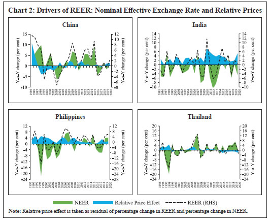
Stylised Facts The real effective exchange rate provides a composite value in the form of exchange rate of a country’s currency vis-a-vis its trading partners which is adjusted for relative price movements. The movement in REER over a period of time shows changes in a country’s trade competitiveness vis-à-vis its trading partners. An increasing REER of a country indicates a rise in the value of its currency vis-à-vis trading partners (trading partners will pay more for buying domestic goods) and thus, a loss of competitiveness. As it is computed against a basket of currencies and adjusted for price differences, REER is usually less volatile than the bilateral nominal exchange rate and shows a steady pattern over medium to long-term. Nevertheless, macroeconomic and financial shocks influence short-term trend in REER (Chart 1). For example, most of the EMEs, barring India and China, witnessed sharp depreciation in their REER in 1998 following the East Asian crisis. Korea and South Africa recorded sharp depreciation in their REER during global financial crisis while Brazil, India, Indonesia and South Africa witnessed a sharp fall in their REER during the taper tantrum period in 2013. Apart from macroeconomic shocks, movement in a country’s real exchange rate is driven by price differentials vis-à-vis its trading partners. Thus, changes in REER can be decomposed into nominal effective exchange rate (NEER) and relative price effect (Chart 2). As depicted in Chart 2, movements in REER in China, Philippines and Thailand in post-2010 period are driven mainly by nominal effective exchange rates. In contrast, trend in variations of India’s REER was contributed largely by relative price effect. 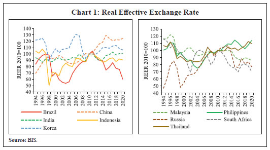
 While the impact of macro-financial shocks and cyclical factors is usually short-lived, long-term trend in REER could be reflective of structural changes taking place in the economy. One of the important factors driving long-term trend of REER is the changes in productivity level of the economy’s tradable sector. For example, an increase in labour productivity of a country causes output per worker to increase at a faster pace vis-à-vis its trading partner which leads to an increase in REER of its currency. China, India, Indonesia, Philippines and Thailand recorded increase in their REERs, whereas Brazil, Russia and South Africa witnessed decrease in their REER during the post-2010 period (Chart 1). The increase in REER of these countries (China, India and Indonesia) coincided with higher growth in their relative per capita GDP (Chart 3). Further, higher productivity growth of China and India is also reflected in their rising share in world exports (Chart 4). 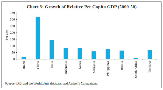 According to the World Bank (2020), the sharp increase in the share of emerging market and developing economies (EMDEs) in world GDP post- 20001 coincided with their higher productivity growth during 2003-08 at around 5 per cent as compared to that of 2 per cent in advanced economies. Further, the World Bank (2020) observed that “In some large EMDEs, such as China and India, productivity is growing substantially faster than in advanced economies…..”. Both China and India witnessed higher growth of labour productivity as well as the total factor productivity (TFP). However, China witnessed relatively higher productivity growth (both labour productivity and TFP). Further, the improvement in productivity began much earlier in China (mid-1980s) than in India (mid-1990s). In 2000s, a few other EMEs such as Malaysia, Philippines, Russia and Thailand intermittently posted higher TFP and labour productivity growth than the advanced economies. IMF (2011) pointed out that a large part of the increase in global trade over long-term horizon was driven by rapidly growing EMEs. It is also observed that trade expansion took place in high-technology products like computers, and the subsequent shift of technology content towards EMEs had implications for relative price changes; and countries with higher level of income embodied in exports witnessed higher growth of per capita GDP. Consequently, EMEs witnessed higher inflation than the advanced economies even though the gap is converging since mid-1990s due to growing emphasis on price stability as evident from the adoption of inflation targeting by EME central banks. 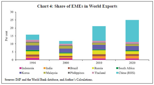 Section III
Review of Literature The purchasing power parity (PPP) theory postulates that the equilibrium exchange rate between two countries is determined by their respective purchasing powers, i.e., inflation. The PPP theory is based on the “law of one price” which argues that in frictionless markets (no tariffs or other trade barriers), where there are no transaction/transportation costs, the price of an identical tradeable commodity is same across countries. In other words, consumer in every country will have the same purchasing power measured in common currency, implying that the relative price levels determine the real exchange rate (Equation 1). where, ‘E’ denotes real exchange rate, ‘e’ is nominal exchange rate, ‘Pf’ represents foreign price level and ‘P’ is domestic price level. Monetary approach to the exchange rate stresses that excess money supply, output and interest rate relative to foreign economy drive nominal exchange rate. Real interest parity implies that differences in nominal interest rates equal the difference in expected inflation plus expected percentage change in real exchange rate. Another theory which provides an explanation of exchange rate movements is the Balassa-Samuelson effect (Balassa, 1964; Samuelson, 1964). It argues that productivity gains in the tradable sector lead to higher wages which gets generalised in the non-tradable sector, thereby causing an increase in inflation and therefore, an appreciation of the real exchange rate of domestic currency. In practice, however, several other factors – both domestic and external – have their influence on the behaviour of real exchange rate. Such factors include the demand side of the economy, country risk premium and capital flows. For example, the concept of Fundamental Equilibrium Exchange Rate (FEER) postulated by Williamson (1994) states that the equilibrium exchange rate will be determined by internal balance characterised by full employment level of output and low and stable inflation, and external balance, i.e., sustainability of balance of payments in the medium term. Internal balance is achieved by changes in REER driven by productivity differences, while external balance is achieved through the impact of the REER on current account. Therefore, if the current account balance is unsustainable, the REER will depreciate, and it will improve the current account balance to a sustainable level. Extending the FEER approach, MacDonald (1997) and Clark and MacDonald (1998) proposed BEER model based on theoretical underpinning of uncovered interest rate parity (UIP). Clark and MacDonald (1998) include relative price of non-traded to traded goods (tnt), net foreign assets (nfa), terms of trade (tot), short-term interest rate differentials (r-r*) and the risk premium component represented by public debt (gdebt/gdebt*), as determinants of the real exchange rate (Equation 2).  where ‘r’ stands for domestic real interest rate and ‘r*’ is world real interest rate, ‘gdebt’ is government debt as a ratio to GDP and ‘gdebt*’ is foreign government debt as a ratio to foreign GDP. ‘tot’ represents terms of trade, ‘tnt’ stands for relative price of non-traded to traded goods and ‘nfa’ denotes net foreign assets of a country (external assets – external liabilities). In view of the policy implications for global trade and development, real exchange rates are monitored and analysed by policymakers, multilateral organisations as well as by the research institutions. For example, the IMF provides an assessment of equilibrium REER of major AEs and EMEs in its External Sector Report by using External Balance Assessment (EBA) methodology, which consists of three approaches. These include the current account (CA) approach, real effective exchange rate (REER) regression and the external sustainability approach.2 However, some studies criticise that the sustainable current account argued in models such as FEER or the IMF’s EBA put extra layer of judgement of calculating current account elasticity (MacDonald, 2000; Grekou 2018). The Centre d’Etudes Prospectives et d’Informations Internationales (CEPII) France estimates the equilibrium REER and misalignment (Actual REER – Equilibrium REER) for all countries based on determinants such as proxy of Balassa-Samuelson (BS) effect, net foreign assets, terms of trade and trade openness (Couharde et al., 2017) and provides country-wise data on proxies of BS effect, viz., per capita GDP, GDP per worker, and consumer price index (CPI) to producer price index (PPI) ratio. The Institute of International Finance (IIF) provides an update of its exchange rate assessment based on FEER model. Empirical literature suggests that studies consider per capita GDP or labour productivity or CPI to PPI ratio as determinants of real exchange rate along with other variables such as terms of trade, and net foreign assets or net capital flows (Lane and Milesi-Ferretti, 2004; Coudert et al, 2013). Some studies have also considered other determinants such as trade openness or trade balance (Maeso-Fernandez et al., 2004; Hossfeld, 2010; and Hajek, 2016), and government expenditure or public debt (Clark and MacDonald, 1998; Maeso-Fernandez et al., 2004; Ricci et al., 2008; Hossfeld, 2010; Bussière et al., 2010; Mancini-Griffolo et al., 2014; and Adler and Grisse, 2014) to assess the role of demand side factors. Long-term or short-term interest rate differentials have been a relatively new addition to the set of determinants of real exchange rate (Clark and MacDonald, 1998; Maeso-Fernandez et al., 2001; Bénassy-Queré et al., 2009; and Fidora et al., 2017). While most of the studies use short-term interest rate as indicated in BEER model, Maeso- Fernandez et al., 2001 argued for long-term interest rate citing empirical evidence on the absence of equalisation in interest rate differential across countries in the long-run. A few studies have also explored relative trade openness (Griffoli et al. 2015; Fidora et al. 2017), relative terms of trade and relative government expenditure (Fidora et al. 2017) as determinants of real exchange rate. Volatile capital flows and changes in risk aversion in global financial markets also influence exchange rate movements. Therefore, some studies take into account different types of capital flows such as foreign direct investment (FDI), foreign portfolio investment (FPI), and other flows (Joyace and Kamas 2003). In the Indian context, a few studies have analysed the determinants of exchange rate. Patel and Srivastava (1997) considered terms of trade and a few other determinants and found real exchange rate of the Indian rupee appreciating with an increase in capital flows and tariffs protection, and depreciating with an increase in investment/GDP ratio and seigniorage-GDP ratio. Pattanaik (1999) found India’s REER aligned to PPP in the long-run as observed by its mean reversion. The author found that misalignments, i.e., deviations from PPP, are corrected through nominal exchange rate and price movements. While analysing REER of India, Joshi (2006) found the real demand effect (money supply and fiscal deficit together named as real demand effect) to be a fundamental determinant besides relative supply variable (index of industrial production of India relative to industrial countries) and relative nominal shocks (price indices in India relative to industrial countries). Kumar (2010) observed that India’s real exchange rate in the long-run was driven by productivity differentials, external sector openness, terms of trade and net foreign assets. Randive and Burange (2013) found government expenditure, openness, inflation differential, foreign institutional investment and long-term interest rate differential as the drivers of real exchange rate. Recent studies based on panel of EMEs including India (Giannellis and Koukouritakis, 2018) found that real exchange rate was broadly aligned to its equilibrium value determined by net foreign assets, productivity and interest rate differentials. Banerjee and Goyal (2020) analysed REER using determinants such as terms of trade, openness, productivity, and fiscal deficit, and found that China, India and Mexico had higher equilibrium exchange rate in the pre-GFC period, than the post-GFC period. The rate of misalignment of REER remained within the range of +/-5 per cent. Guria and Sokal (2021) found bi-directional causality between productivity differential and REER in India. They pointed out that causality from productivity differentials to REER confirms the Balassa- Samuelson hypothesis, while causality from REER to productivity differentials indicates the impact of appreciation in real exchange rate on the productivity growth3. Section IV
Data and Methodology Among various explanations of movements in REER in the long-run, the BS effect is the most widely accepted determinant. However, we use other possible determinants as suggested in the literature on BEER model. The BEER model considers both structural and temporary factors which influence the real exchange rate. Further, the BEER model does not involve any normative content or judgement while estimating equilibrium exchange rate which is the case with other methodologies such as the IMF’s EBA. Therefore, the recent literature on equilibrium real exchange rate has largely preferred the BEER model (Macdonald and Dias, 2007; Melecký and Komárek, 2007; Fidora et al., 2017; Michele et al., 2020). The advantage of this approach lies in obtaining the equilibrium value directly from empirically estimated model.4 In this paper, the BS effect is proxied by per capita GDP relative to trading partners, while other determinants considered are net foreign assets, terms of trade index, interest rate differentials and debt-GDP ratio. Due to the non-availability of productivity data for traded and non-traded sectors separately, studies mostly use per capita GDP as a proxy of the BS effect.5 As alluded earlier, rise in productivity growth vis-à-vis trading partners is expected to result in an appreciation of the real exchange rate. With regard to the impact of fiscal policy on real exchange rate, studies have considered public expenditure-GDP ratio or the debt-GDP ratio. The increase in public expenditure boosts aggregate demand, which may lead to more imports than exports and therefore, more demand for foreign currency, and eventually the depreciation of real exchange rate. However, if higher expenditure is associated with increased taxes, its impact would be neutralised. The debt position of the current period captures debt financed public expenditure or the excess of expenditure over revenues (debtt = debtt-1 + deficitt). Apart from the impact channelised through demand, an increase in public expenditure results in higher deficit and public debt, which can influence the exchange rates due to higher country risk premium (RBI, 2019). The increase in public debt may cause higher interest rate which may lead to a surge in capital flows and the appreciation of exchange rate. The implications of public debt for country risk premium and interest rate are important for EMEs, particularly for countries like India where debt-GDP ratio is higher than the recommended levels (RBI, 2022). Therefore, we use debt-GDP ratio to assess the impact of fiscal policy on exchange rate. As mentioned earlier, the size of net foreign assets (nfa) is an important determinant considered in empirical literature and is found to be positively associated with REER. Intuitively, higher foreign liabilities increase interest and non-interest payments from the country, necessitating surplus in the current account through currency depreciation to finance additional payments. Improvements in net terms of trade are generally found to be positively associated with real exchange rate due to the income effect being stronger than the substitution effect. Favourable export prices vis-à-vis trading partners increase domestic income to be spent on tradables and non-tradables, which may lead to inflationary pressures. While the prices of tradables are generally externally determined and thus remain largely unaffected, domestic prices of non-tradables generally respond positively to changes in export prices. By contrast, higher export prices may gradually reduce foreign demand for tradable goods and, therefore, resource diversion to non-tradable sectors reduces inflation in the economy which, in turn, causes depreciation in real exchange rate of local currency. Finally, as alluded earlier, short-term interest rate is also argued to be an important determinant of the exchange rate (MacDonald 1997; and Clark and MacDonald 1998). The uncovered interest rate parity theory suggests that high domestic interest rate relative to foreign interest rate would lead to depreciation of domestic currency against foreign currency. In view of the above discussion and following literature on equilibrium exchange rate (Couharde et al., 2017, Fidora et al., 2017, and Giannellis and Koukouritakis, 2018), we consider the following form of BEER model. 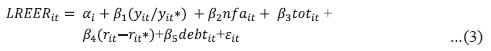 where, LREER is the log of CPI based REER index with base year 2010 obtained from the Bank for International Settlements (BIS). These are weighted indices based on time varying trade weights with 59 trading partners. yit/yit*, i.e., relative per capita GDP, is calculated as: where, yit is the real per capita GDP of country ‘i’ at time ‘t’, and Wij,t is country i’s trade weight for its trading partner ‘j’. yjt is per capita GDP of ‘j’th trading partner at time ‘t’. Thus, foreign per capita GDP (yit*) is represented by weighted average of per capita GDP of 59 trading partners. We have used BIS trade weights matrix of 60 countries to make weights of per capita GDP consistent with those of REER. The data on real per capita GDP (i.e., PPP-adjusted per capita GDP in US dollar) are obtained from the World Bank database. In equation 3, ‘r’ represents domestic real interest rate and r* is foreign real interest rate, and rit-rit* is the interest rate differential between domestic and foreign interest rate. Foreign interest rate is proxied by interest rates in the US. Further, we use two types of interest rates to calculate the interest rate differential – short-term interest rate differential and long-term interest rate differential. For calculating the long-term real interest rate differential, interest rate (lending rates of banks) data are sourced from the World Bank, and the GDP deflators are used to convert them into real interest rate. For calculating the short-term real interest rate differential, money market rate and CPI based inflation data obtained from the IMF are used. Variable ‘nfa’ in equation 3 is net foreign assets as a ratio to GDP. Net foreign assets data are sourced from ‘External Wealth of Nations’ database of Lane and Milesi-Ferretti (2017). Nominal GDP available in World Bank database is used for computing net foreign assets to GDP ratio. ‘tot’ stands for natural logarithm of terms of trade index (June 2012=100) which is obtained from the IMF database (Gruss and Kebhaj 2019). It is the commodity net export price index (weighted by net exports to GDP). ‘debt’ stands for public debt to GDP ratio which is obtained from IMF’s ‘Global Debt Database’, historical debt database and Fiscal Monitor (October 2021). Sample used for empirical estimation in this paper consists of annual data from 1994 to 2020 for ten countries, viz., Brazil, China, India, Indonesia, Korea, Malasiya, Philippines, Russia, South Africa and Thailand. Thus, our sample includes all BRICS countries which account for 24 per cent of world GDP and 16 per cent of world trade, and other major emerging market economies in Asia. Section V
Empirical Results As the choice of econometric method depends largely on time series properties of the data, we checked stationary property of variables by using panel unit root tests, viz., Levin-Lin-Chu (LLC), Im-Pesaran-Shin (IPS) and cross-sectionally augmented IPS (CIPS) test proposed by Pesaran (2007). While the null hypothesis in LLC test assumes common unit root process, in IPS test, the null hypothesis assumes individual unit root process, i.e., all panels contain unit roots. LLC and IPS test are widely used and are first-generation panel unit root test, however, CIPS test which accounts for cross-sectional dependence is considered as second generation panel unit root test. The size of estimated panel unit root test can be affected by the cross-sectional dependence in data (Annex 1) and thus the CIPS test is recommended (Banerjee et. al, 2005). The results of LLC, IPS and CIPS tests are provided in Table 1 which reveal that the null hypothesis of unit root cannot be rejected for log of REER (LREER), relative per capita GDP, terms of trade, debt and net foreign assets, when the variables are used in level form. However, upon first differencing, all these variables are found to be stationary. On the other hand, short-term and long-term interest rate differentials are found to be stationary at levels as well as in the first difference form. Overall, the results indicate that most of the variables are non-stationary at levels in at least one test but all the variables used in the first difference form are found to be stationary in all three tests. Further, the results of cross-sectionally augmented CIPS test are consistent with LLC and IPS tests. In the context of REER, unit root testing assumes special significance as stationary REER can be considered as an evidence of equilibrium exchange rate, if the productivity growth in a country vis-à-vis its trading partners is stable. To ascertain an evidence on the cause-and-effect relationship between LREER and its potential determinants, causality test developed by Dumitrescu and Hurlin (2012) is undertaken. The null hypothesis (H0) in Dumitrescu and Hurlin test is ‘no causal relationship’. The results of causality test shown in Annex 2 indicates unidirectional causality running from relative per capita GDP (yit/yit*), terms of trade (tot), public debt (debt) and interest rate differential (ST_USA) to log of REER (LREER). However, there is an evidence of bi-directional causality between net foreign assets (nfa) and LREER which is possibly reflecting J-curve effect as the stock of net foreign assets is largely a reflection of accumulation of current account balance6. In view of the above results of panel unit root tests, we examine the long-run relationship of REER with its macroeconomic fundamentals. Accordingly, we use panel cointegration tests developed by Kao (1999), Pedroni (1999 and 2004) and Westerlund (2007). Westerlund (2007) test differs from the other two tests in terms of the alternative hypothesis i.e., ‘some panels are cointegrated’, as against the alternative hypothesis ‘all panels are cointegrated’ in Kao (1999) and Pedroni (1999 and 2004) tests. Further, the Westerlund test is error-correction based and accounts for possible cross-sectional dependence (Cheik and Cheik, 2013). In our baseline model, all the three tests confirm cointegration, suggesting the presence of a long-run equilibrium relationship between REER and relative per capita GDP in EMEs (Table 2). In the next step, we augment our model sequentially by incorporating additional variables in alternative specifications. The presence of cointegrating relationship between REER and its determinants is observed across all the augmented specifications. In the most augmented model, the cointegration between LREER and other variables such as net foreign assets, terms of trade, interest rate differential and debt-GDP ratio has been confirmed. Table 1: Results of Panel Unit Root Tests
(Sample period: 1994-2020) | | Variable | Level | First difference | | LLC t statistic | IPS W statistics | CIPS T statistic | LLC t statistic | IPS W statistic | CIPS T statistic | | LREER | -0.39 | -1.27 | -1.93 | -4.74*** | -5.57*** | -3.06*** | | yit/yit* | 3.52 | 0.63 | -1.21 | -1.75** | -3.05*** | -3.04** | | | (1.00) | (0.74) | | (0.04) | (0.00) | | | tot | 0.07 | 0.29 | -1.37 | -1.86** | -3.53*** | -4.37*** | | | (0.53) | (0.61) | | (0.03) | (0.00) | | | nfa | 0.06 | 1.22 | -1.67 | -2.94*** | -5.40*** | -3.27*** | | | (0.52) | (0.89) | | (0.00) | (0.00) | | | debt | 1.81 | -0.77 | -0.93 | -5.87*** | -2.88*** | -3.09*** | | | (0.97) | (0.22) | | (0.00) | (0.00) | | | ST_USA | -6.16*** | -3.74*** | -2.88*** | -16.59*** | -10.93*** | -9.08*** | | | (0.00) | (0.00) | | (0.00) | (0.00) | | | LT_USA | -4.57*** | -4.61*** | -3.87*** | -12.64*** | -8.04*** | -5.36*** | | | (0.00) | (0.00) | | (0.00) | (0.00) | | LLC: Levin-Lin-Chu (2002); IPS: Im-Pesaran-Shin (2003); CIPS: Cross-sectionally augmented IPS ***, **, * indicate statistical significance at 1 per cent, 5 per cent and 10 per cent levels, respectively.
Note: 1. For the LLC test, the null hypothesis is ‘panels contain unit roots’; for the IPS and CIPS it is ‘all panels contain unit roots’.
2. Lag length selection based on AIC.
3. ST_USA: Short-term real interest rate differential with USA; and LT_USA: Long-term real interest rate differential with USA. |
| Table 2: Panel Cointegration Test Results | | Variables | Kao test ADF | Pedroni test | Westerlund Test | | Within-dimension (Panel) | Between-dimension (Group) | | t-statistic | Panel v-Statistic | Panel rho- statistic | Panel PP t statistic | Panel ADF t tatistics | Group rho- statistic | Group PP t statistic | Group ADF t tatistics | Variance Ratio statistic | | LREER, yit/yit* | -3.33*** | 4.16*** | -2.82*** | -3.38*** | -3.97*** | -1.05 | -2.88*** | -4.26*** | -2.02** | | LREER, yit/yit*, nfa | -3.31*** | 3.88*** | -2.34*** | -4.14*** | -4.50*** | -0.35 | -3.03*** | -3.89*** | -1.88** | | LREER, yit/yit*, nfa, tot | -3.54*** | 2.91*** | -1.05 | -2.84*** | -3.51*** | 0.77 | -2.15** | -3.61*** | -2.24*** | | LREER, yit/yit*, nfa, tot, debt | -3.93*** | 2.11** | -0.33 | -4.12*** | -5.39*** | 1.43 | -5.90*** | -6.16*** | -2.18*** | | LREER, yit/yit*, nfa, tot, debt, ST_USA | -4.04*** | 0.90 | 0.81 | -3.48*** | -3.21*** | 2.31 | -4.44*** | -4.81*** | -1.76** | | LREER, yit/yit*, nfa, tot, debt, LT_USA | -4.08*** | 0.59 | 0.99 | -3.10** | -4.37*** | 2.43 | -3.39*** | -4.53*** | -1.53* | | Note: ***, **,* indicate statistical significance at 1 per cent, 5 per cent and 10 per cent levels, respectively. | After confirming cointegration, panel Dynamic Ordinary Least Square (DOLS) model is estimated to obtain the coefficient of each determinant (Table 3). Fully Modified Ordinary Least Square (FMOLS) method proposed by Phillips and Hansen (1990) or DOLS proposed by Stock and Watson (1993) are consistent in the event of endogeneity and serial correlation as against potentially inconsistent OLS. Kao and Chiang (2000), Mark and Sul (1999, 2003), and Pedroni (2001) proposed extensions of DOLS estimator to panel data settings. While FMOLS follows a non-parametric approach, panel DOLS uses cross-section specific leads and lags of first difference of independent variables to take care of asymptotic serial correlation and endogeneity. While estimating DOLS, pooled (weighted) estimator is chosen which also accounts for heterogeneity across cross-sections. It uses cross-section specific estimates of the conditional long-run residual variances to reweight the moments for each cross-section. As a robustness check of the empirical results, FMOLS estimator is also used (Table 3). Further, due to a mix of stationary and non-stationary variables (interest rate differential is found to be stationary both at levels and in first differenced form), panel ARDL model is applied as an additional ‘safety net’ (Table 4). | Table 3: Determinants of REER - Results of DOLS/FMOLS estimation | | Model | DOLS | FMOLS | DOLS | FMOLS | DOLS | FMOLS | DOLS | FMOLS | DOLS | FMOLS | | 1 | 2 | 3 | 4 | 5 | 6 | 7 | 8 | 9 | 10 | | yit/yit* | 1.99*** | 1.72*** | 2.24*** | 1.92*** | 2.36*** | 1.85*** | 1.09*** | 1.43*** | 1.43*** | 1.44*** | | | (7.44) | (4.02) | (5.76) | (6.31) | (6.33) | (7.61) | (3.27) | (5.37) | (5.94) | (10.06) | | nfa | | | 0.39*** | 0.42*** | 0.41*** | 0.41*** | 0.40*** | 0.33*** | 0.59*** | 0.33*** | | | | | (4.16) | (4.07) | (3.54) | (4.98) | (3.26) | (4.11) | (7.87) | (8.31) | | tot | | | | | 0.90** | 1.23*** | 0.81** | 0.87*** | 0.99*** | 0.89*** | | | | | | | (2.08) | (4.11) | (2.18) | (2.91) | (3.70) | (5.61) | | debt | | | | | | | -0.003** | -0.003*** | -0.003** | -0.002** | | | | | | | | | (-2.85) | (-3.57) | (-3.99) | (-5.12) | | ST_USA | | | | | | | | | 0.02*** | 0.003*** | | | | | | | | | | | (7.70) | (4.15) | | R2 | 0.71 | 0.65 | 0.81 | 0.68 | 0.87 | 0.71 | 0.94 | 0.73 | 0.95 | 0.77 | | Adjusted R2 | 0.61 | 0.61 | 0.70 | 0.64 | 0.74 | 0.67 | 0.82 | 0.69 | 0.80 | 0.74 | Note: 1. Figures in brackets are t-statistics.
2. ***,** and * indicates statistical significance at 1 per cent, 5 per cent and 10 per cent levels, respectively. | In Table 3, columns 1 and 2 provide results of the baseline model where relative per capita GDP (yit/yit*) is the only explanatory variable of REER. Per capita GDP is found to be a significant determinant of REER, both statistically and numerically. This finding is consistent with higher productivity growth of EMEs than that of AEs as explained in section II and thus it indicates the presence of the BS effect. In the next step, the model is augmented to include net foreign assets (columns 3 and 4). The coefficient of net foreign assets (nfa) is having an expected sign and it is statistically significant. Further, the coefficient of terms of trade (tot) added with per capita GDP and nfa (columns 5 and 6) is found to be statistically significant. This was followed by adding debt to GDP ratio as an additional determinant. An increase in debt to GDP ratio, as a priori expected, is found to have a depreciating effect on REER (columns 7 and 8), substantiating the inverse relationship between the two, possibly reflecting the adverse effects on exchange rate channelised through (i) expansionary fiscal policy, and (ii) country risk premium. Finally, to examine the impact of interest rate differentials, we use two proxies of real interest rate differentials, viz., short-term interest rate differential with USA (ST_USA), and long-term interest rate differential with USA (LT_USA). However, only short-term real interest rate differential with USA is found to be statistically significant. The results of FMOLS and DOLS with respect to the sign and magnitude of independent variables in explaining REER are broadly similar. Further, due to stationarity properties of interest rate differentials, empirical estimation using the panel ARDL model as proposed by Pesaran et al. (1999) for the same set of dependent and explanatory variables is undertaken. The coefficients of most of the variables are broadly similar in terms of the sign, their magrnitude and the statistical significance (Table 4). The error correction term of panel ARDL model is found to be negative and statistically significant. | Table 4: Results of ARDL Model | | Variables | 1 | 2 | 3 | 4 | 5 | | yit/yit* | 2.22*** | 3.26*** | 3.46*** | 1.89*** | 1.30*** | | | (6.51) | (9.77) | (11.71) | (7.44) | (5.19) | | nfa | | 0.64*** | 0.60*** | 0.27*** | 0.32*** | | | | (9.37) | (10.82) | (4.33) | (5.11) | | tot | | | 0.68* | 0.19 | 0.53** | | | | | (1.89) | (0.77) | (2.21) | | debt | | | | -0.004*** | -0.005*** | | | | | | (-6.78) | (-7.91) | | ST_USA | | | | | 0.004** | | | | | | | (2.03) | | Error correction term | -0.43*** | -0.48*** | -0.50*** | -0.57*** | -0.51*** | | | (-7.91) | (-4.07) | (-3.96) | (-4.94) | (-5.68) | Note: 1. ***, ** and * indicate statistical significance at 1 per cent, 5 per cent and 10 per cent levels, respectively.
2. Figures in brackets are t-statistics. | Section VI
Trend in Equilibrium REER and the Extent of Misalignments As alluded earlier, overvaluation or undervaluation of the real exchange rate of EME currencies has always attracted attention of policymakers. Persistent undervaluation of exchange rate is considered as a mercantilist policy where a country by intervening in the foreign exchange market devalues exchange rate for export promotion. On the other hand, overvaluation of exchange rate such as during surges in capital inflows adversely affects exports and domestic employment. Therefore, an assessment of exchange rate compared to its equilibrium value assumes importance. Predicted value obtained from estimated model as given in column 9 in Table 3 is considered as equilibrium REER level which is compared with actual REER to assess the extent of misalignment of each currency.7 Accordingly, the difference between the actual REER and the equilibrium REER is called as misalignments i.e., overvaluation or undervaluation. Misalignment = Actual REER – Equilibrium REER
Overvaluation = Actual REER > Equilibrium REER
Undervaluation = Actual REER < Equilibrium REER The comparison of actual and equilibrium values as shown in Chart 5 provides several attributes of REER behaviour in EMEs. First, the trend in actual REER in most of the sample countries is in sync with their respective paths of equilibrium values implying exchange rate being driven by macroeconomic fundamentals (Chart 5). Second, the diverging trend in equilibrium REER across the EMEs (i.e., equilibrium REER increased in some countries and decreased in other countries) over the sample period is largely showing an impact of structural changes, viz., productivity growth, confirming presence of the BS effect among EMEs. For example, uptrend in both actual and equilibrium REER in China, India, Philippines and Thailand is in line with their higher relative per capita GDP growth. On the other hand, South Africa and Brazil which witnessed lower growth in their relative per capita GDP also recorded decline in their actual and equilibrium REER. Third, misalignment of REER i.e., deviation from equilibrium value, is lower and remained range-bound at around 2-3 per cent. Fourth, the misalignment is asymmetric across EMEs. For example, actual REER of China, Philippines and Thailand during 2000s generally remained lower than the equilibrium values, while in India and South Africa, it remained above the equilibrium level. The countries experiencing overvaluation in post-GFC years, viz., Brazil, India and Philippines recorded relatively higher inflation, while those having undervaluation, viz., China and Korea, recorded relatively lower inflation. In view of this, the REER misalignment [defined as, log (REER) – log (equilibrium REER)] was regressed upon changes in log of NEER and change in relative prices. Results based on panel ordinary least square estimation shown in Annex 3 indicate that the REER misalignment in EMEs is driven by changes in NEER. However, country-specific regressions indicate that the change in relative prices (vis-à-vis trading partners) is the major factor leading to misalignment in Brazil and India. On the other hand, the NEER is found to influence REER’s misalignment in Philippines and South Africa. Fifth, EMEs witnessed sharp movements in both actual and equilibrium REER during macro-financial shocks such as the East Asian Crisis and the Global Financial Crisis. These results with respect to equilibrium REER and the rate of misalignment are broadly similar to Giannellis and Koukouritakis (2018) and Banerjee and Goyal (2020).  Section VII
Conclusion Against the backdrop of inconclusive empirical evidence in the literature with regard to the equilibrium exchange rate, this paper provides an estimate of equilibrium REER for select EMEs. Using annual data from 1994 to 2020 for ten EMEs, the paper finds that persistent appreciation/ depreciation in REER in the long-run is consistent with the equilibrium level as determined by macroeconomic fundamentals. For example, an increase in the level of the equilibrium REER in some countries reflects the presence of the Balassa-Samuelson effect. Improvements in net terms of trade and net foreign assets are found to cause REER appreciation. However, expansionary fiscal policies may be associated with higher country-risk premium, as evident from an inverse relationship between debt-GDP ratio and REER. The impact of interest rate differential is found to be positive. The comparison of actual and equilibrium REER levels suggests that the REER is being determined by macroeconomic fundamentals and the misalignment (overvaluation/undervaluation) is usually within a narrow range of +/- 3 per cent. Like most EMEs, India’s REER also showed two-way movements around its equilibrium value, implying no evidence of currency manipulation or mercantilist undervaluation. Thus, the observed upward co-movements of actual and equilibrium REER in some EMEs like India and China shows the productivity driven increase in REER, which is not a sign of loss of external competitiveness. References: Adler K. & Grisse C. (2014). Real exchange rates and fundamentals: Robustness across alternative model specifications. SNB Working Papers No 7. Balassa, B. (1964). The purchasing-power parity doctrine: A reappraisal. Journal of Political Economy, 72 (6): 584-596. Banerjee K. & Goyal A. (2020). Equilibrium real exchange rates and misalignments in large emerging markets: A re-look through panel cointegrating estimation. IGIDR working paper No 001. Banerjee, A., Marcellino, M. & Osbat, C. (2005). Testing for PPP: Should we use panel methods?. Empirical Economics, Volume 30, 77–91. Bénassy-Queré, A., Béreau, S. & Mignon, V. (2009). Robust estimations of equilibrium exchange rates within the G20: A panel BEER approach. Scottish Journal of Political Economy, 56(5): 608-633. Bussière, M., Ca’Zorzi, M., Chudik, A. & Dieppe, A. (2010). Methodological advances in the assessment of equilibrium exchange rates. ECB Working Paper No 1151. Cheikh, B. N. & Cheikh M. H. (2013). A Panel Cointegration Analysis of the Exchange Rate Pas-through, Economics Bulletin, Vol. 33, Issue 4, 2778-90. Choi, I. (2001). Unit root test for panel data. Journal of International Money and Finance, 20(2), 249-72. Clark, P.B. & MacDonald, R. (1998). Exchange rates and economic fundamentals: A methodological comparison of BEERs and FEERs. IMF Working Papers No. 67. Coudert, V., Couharde, C. & Mignon, V. (2013). On currency misalignments within the Euro area. Review of International Economics 21(1). Couharde, C., Delatte, A.-L., Grekou, C., Mignon, V. & Morvillier, F. (2017). Eqchange: A world database on actual and equilibrium effective exchange rates. CEPR Discussion Papers No. 12190. Cubeddu L., Krogstrup S., Adler G., Rabanal P., Dao M. C., Hannan S. A., Juvenal L., Li N., Buitron C. O., Rebillard C., Garcia-Macia D., Jones C., Rodriguez, J. Chang K. S., Gautam D., & Wang Z. (2019). The external balance assessment methodology: 2018 update. IMF working paper No. 65. Dumitrescu, E.-I., & Hurlin, C. (2012). Testing for Granger Non-causality in Heterogeneous Panels. Economic Modelling, Vol. 29 (4): 1450–1460. Fidora, M., Giordano, C. & Schmitz M. (2017). Real exchange rate misalignments in the Euro area. ECB Working Paper No. 2108. Giannellis N. & Koukouritakis, M. (2018). Currency misalignments in the BRIICS countries: Fixed Vs. floating exchange rates. Open Economies Review, Vol. (29):1123-51. Grekou C. (2018). Currency misalignments and economic growth: The foreign currency-denominated debt channel. CEPII Working Paper No 12 Griffoli, T.M., Meyer, C., & Natal, J. (2015). Determinants of the Swiss Franc real exchange rate. Swiss Journal of Economics Statistics Vol. 151 (4): 299- 331. Gruss, B., & Suhaib Kebhaj. (2019). Commodity terms of trade: A new database. IMF Working Paper No. 21. Gubler, M. & Sax, C. (2019). The Balassa-Samuelson effect reversed: new evidence from OECD countries. Swiss Journal of Economics and Statistics, Vol. 155, No 3 Guria, J. & Sokal S. (2021). Effective exchange rate indices of the Indian Rupee. RBI Bulletin, January. Hajek, J. (2016). Real exchange rate misalignment in the Euro area: Is the current development helpful?’. Charles University Prague, Institute of Economic Studies Working Paper No. 11. Hossfeld, O. (2010). Equilibrium real effective exchange rates and real exchange rate misalignments: Time series vs. panel estimates. FIW Working Paper No. 65. Im, K. S., Pesaran, H., & Shin, Y. (2003). Testing for unit roots in heterogeneous panels. Journal of Econometrics, 115(1), 53–74. IMF (2011). Changing patterns of global trade. Policy Papers, Volume 2011/044 IMF (2020). Fiscal Monitor. April 2020. Joshi, H. (2006). The fundamental equilibrium real exchange rate in India: An approach to estimation and measurement of misalignment. Reserve Bank of India Occasional Papers Vol. 27 (3):1-24. Joyce, J. & Kamas, L (2003). Real and nominal determinants of real exchange rates in Latin America: Short-run dynamics and long-run equilibrium. Journal of Development Studies Vol. 39 (6): 155-182, Kao, C. (1999). Spurious regression and residual-based tests for cointegration in panel data. Journal of Econometrics 90 (1): 1-44. Kao, C. & Chiang M (2000). On the estimation and inference of a cointegrated regression in panel data. in Baltagi, B. H. et al. eds., Nonstationary Panels, Panel Cointegration and Dynamic Panels, 15, Amsterdam: Elsevier, 179–222. Kumar, S. (2010). Determinants of real exchange rate in India: An ARDL approach. Reserve Bank of India Occasional Papers, Vol. 31, No.1. Lane, P. R. & Milesi-Ferretti, G.M. (2004). The transfer problem revisited: Net foreign assets and real exchange rates. The Review of Economics and Statistics 86(4): 841-857. Lane P. R. & Milesi-Ferretti G. M. (2017). The external wealth of nations revisited: International financial integration in the aftermath of the global financial crisis. IMF Economic Review, 66, 189-222 Levin, A., Lin, C., & Chu, C. J. (2002). Unit root tests in panel data: Asymptotic and finite sample properties. Journal of Econometrics, 108(1), 1–24. Lin S. (1994). Government debt and the real exchange rate in an overlapping generations model. Journal of Economic Integration, 9 (1), 94-105. MacDonald, R. (1997). What determines real exchange rate? The long and short of it”. IMF Working Paper No. 21. MacDonald, R. (2000). Concepts to calculate equilibrium exchange rates: An overview. Bundesbank Series 1 Discussion Paper No. 03, Available at SSRN: https://ssrn.com/abstract=2785109 or http://dx.doi.org/10.2139/ssrn.2785109 MacDonald, R. & Dias P. (2007). Behavioural equilibrium exchange rate estimates and implied exchange rate adjustments for ten countries. Paper prepared for the workshop on Global Imbalances, Peterson Institute of International Economics, Washington DC available at https://www.gla.ac.uk/media/Media_30667_smxx.pdf Maddala, G.S., & Wu, S. (1999). A comparative study of unit root tests with panel data and a new simple test. Oxford Bulletin of Economics and Statistics, 61, 631-52. Maeso-Fernández, F., Osbat, C. & Schnatz, B. (2001). Determinants of the Euro real effective exchange rate: A BEER/PEER approach. ECB Working Paper No. 85. Maeso Fernández, F., Osbat, C. & Schnatz, B. (2004). Towards the estimation of equilibrium exchange rates for CEE acceding countries: Methodological issues and a panel cointegration perspective. ECB Working Paper No. 353. Mancini-Griffolo, T., Meyer, C., Natal, J-M & Zanetti, A. (2014). Determinants of the Swiss franc real exchange rate. SNB Working Paper No. 8. Mark, N. C. & Sul, D. (1999). A computationally simple cointegration vector estimator for panel data. Ohio State University manuscript available at http://citeseerx.ist.psu.edu/viewdoc/summary?doi=10.1.1.46.5610 Mark, N. C. & Sul D. (2003). Cointegration vector estimation by panel DOLS and long-run money demand. Oxford Bulletin of Economics and Statistics, 65, 655–680. Melecký, M. & Komárek, L. (2007). The behavioural equilibrium exchange rate of the Czech Koruna. Transition Studies Review 14, pp. 105-121. Michele, C., Cap A., Mijakovic A., & Rubaszek M. (2020). The predictive power of equilibrium exchange rate models. ECB Working Paper No. 2358. Mohanty, D. (2013). Interest rates and economic activity. Speech delivered to the Association of Financial Professionals of India (AFPI), Pune, on August 23, 2013. Patel U. R. & Srivastava P. (1997). Some implications of real exchange rate targeting in India. ICRIER working paper. Available at https://icrier.org/pdf/Srivastava.pdf Patnaik I. & Pauly P. (2001). The Indian foreign exchange market and the equilibrium real exchange rate of the rupee. Global Business Review 2(2). Pattanaik S (1999). REER: The leading indicator. Reserve Bank of India Occasional Papers Vol. 20, No. 2. Pedroni, P. (1999). Critical values for cointegration tests in heterogeneous panels with multiple regressors. Oxford Bulletin of Economics and Statistics, 61 (S1): 653-670. Pedroni, P. (2001). Purchasing power parity tests in cointegrated panels. The Review of Economics and Statistics, 83, 727–731. Pedroni, P. (2004). Panel cointegration, asymptotic and finite sample properties of pooled time series tests with an application to the PPP hypothesis. Econometric Theory, 20(3): 597-625 Pesaran, M.H., Shin, Y., & Smith, R.P. (1999). Pooled mean group estimation of dynamic heterogeneous panels. Journal of the American Statistical Association, Vol. 94, No. 446, 621-634. Pesaran, M. H. (2007). A simple panel unit root test in the presence of crosssection dependence. Journal of Applied Econometrics, Vol. 22, No. 2, 265- 312. Phillips, P.C.B. & Hansen, B.E., (1990). Statistical inference in instrumental variables regression with I (1) processes. Review of Economic Studies, Vol. 57, No.1, pp.99–125. Randive R. R. & Burange L. G. (2013). The determinants of India’s real exchange rate: An ARDL approach. The India Economic Journal, 61(3):407- 28. Reserve Bank of India (RBI) (2019). Estimable fiscal multipliers for India. Monetary Policy Report, April 2019: 35-37. Reserve Bank of India (RBI) (2022). Report on Currency and Finance, 2021-22. Ricci, L.A., Milesi-Ferretti, G.M. & Lee, J. (2008). Real exchange rates and fundamentals: a cross-country perspective. IMF Working Paper No. 13. Samuelson, P.A. (1964). Theoretical notes on trade problems. Review of Economics and Statistics, Vol. 46 (2): 145-154. Stock, J. H. & Watson M. (1993). A simple estimator of cointegrating vectors in higher order integrated systems. Econometrica, 61, 783-820. Tica, J. & Druzic, I. (2006). The Harrod-Balassa-Samuelson effect: a survey of empirical evidence. University of Zagreb, Faculty of Economics and Business, Working Paper No. 06-7/686. Westerlund, J. (2007). Testing for error correction in panel data. Oxford Bulletin of Economics and Statistics. Vol. 69, Issue 6, 709–748. Williamson, J. (1994). Estimates of FEERs. in J. Williamson ed., Estimating Equilibrium Exchange Rates, Institute for International Economics, Washington, D.C. World Bank (2020). Global productivity trends, drivers and policies. Edited by Alistair Dieppe, Washington DC.
| Annex 1: Cross-Sectional Dependence Test | | Variable | Breusch-Pagan LM Test | Pesaran Scaled LM Test | Bias-Corrected Scaled LM Test | Pesaran CD | | LREER | 191.79*** | 15.47*** | 15.28*** | 6.06*** | | yit/yit* | 946.61*** | 95.04*** | 94.85*** | 30.52*** | | tot | 762.24*** | 75.60*** | 75.41*** | -1.10 | | nfa | 355.55*** | 32.73*** | 32.54*** | 9.51*** | | debt | 282.78*** | 25.06*** | 24.87*** | 4.00*** | | ST_USA | 131.52*** | 9.12*** | 8.93*** | 2.81*** | | LT_USA | 144.93*** | 10.53*** | 10.34*** | 4.55*** | *** indicate statistical significance at 1 per cent level.
Note: ST_USA: Short-term real interest rate differential with USA; and LT_USA: Long-term real interest rate differential with USA. |
| Annex 2: Panel Causality Test Results | | Null Hypothesis | Pair-wise Dumitrescu and Hurlin Panel Causality Tests | | W-statistic | Z-bar statistic | P-Value | | Relative per capita GDP (yit/yit*) does not homogeneously cause LREER | 6.09 | 4.93 | 0.00 | | LEER does not homogeneously cause Relative per capita GDP (yit/yit*) | 1.66 | -0.72 | 0.47 | | nfa does not homogeneously cause LREER | 7.68 | 6.94 | 0.00 | | LREER does not homogeneously cause nfa | 5.50 | 4.17 | 0.00 | | tot does not homogeneously cause LREER | 3.75 | 1.95 | 0.05 | | LREER does not homogeneously cause tot | 2.28 | 0.08 | 0.94 | | debt does not homogeneously cause LREER | 8.86 | 8.44 | 0.00 | | LREER does not homogeneously cause debt | 1.71 | -0.65 | 0.51 | | ST_USA does not cause homogeneously LREER | 9.30 | 9.01 | 0.00 | | LREER does not homogeneously cause ST_USA | 2.73 | 0.65 | 0.52 | | Notes: lag length (2 lags) is selected based on AIC. |
Annex 3: Results of drivers of misalignment
[Dependent variable misalignment = log (REER) – log (equilibrium REER)] | | Panel of 10 countries | | | Change in log(NEER) | Change in relative prices | Constant | | | 0.11** | 0.07 | 0.003 | | | (2.40) | (1.06) | (0.58) | | Cross-Section specific coefficients | | Country | Change in log(NEER) | Change in relative prices | Constant | | Brazil | 0.22 | 0.35** | -0.001*** | | | (1.34) | (2.45) | (0.04) | | China | 0.32 | -0.43 | -0.007 | | | (1.31) | (-0.62) | (-0.43) | | India | 0.07 | 0.67*** | -0.005 | | | (0.44) | (2.87) | (-0.51) | | Indonesia | 0.09 | 0.04 | 0.007 | | | (1.19) | (0.25) | (0.59) | | Korea | 0.10 | -0.18 | 0.002 | | | (0.40) | (-0.11) | (0.01) | | Malaysia | 0.23 | -1.52 | 0.004 | | | (1.24) | (-1.59) | (0.38) | | Philippines | 0.37* | 0.47 | -0.001 | | | (1.89) | (0.55) | (-0.05) | | Russia | -0.11 | -0.23 | 0.02 | | | (-0.73) | (-1.32) | (0.78) | | South Africa | -0.26** | -0.40 | 0.001 | | | (-2.26) | (-0.62) | (0.03) | | Thailand | 0.19 | 0.90 | -0.001 | | | (0.84) | (1.09) | (-0.16) | Note: 1. ***, ** and * indicate statistical significance at 1 per cent, 5 per cent and 10 per cent levels, respectively.
2. Figures in brackets are t-statistics. |
|