R. K. Sinha^*

Received on: January 14, 2022
Accepted on: May 02, 2022

A reliable assessment of the future pension liabilities of any enterprise is critical to the overall enterprise risk management. For banks, in particular, information on the estimated quantum of variations in pension liabilities is useful for pro-active and prudent provisioning, which can have a long-term bearing on their balance sheets. The paper constructs salary indices for the Indian banking sector for the period 1987 to 2022 and provides a framework to decompose the rise in salary indices as a result of three components viz., compensation for inflation, real increase that raises the purchasing power of salary, and rewarding merit. The indices are projected for the future and then used to compute benefits using the “Indian Assured Lives Mortality Table 2012-14 Ultimate” tables, enabling valuation (estimation) of various contingent liabilities of banks. The paper provides scenarios to assess the impact on employers’ pension liabilities in future due to variations in key assumptions viz., salary scales, decrement rates (mortality and attrition), and interest rate.

JEL Classification: J26, J31, J32, H55

Keywords: Actuarial present value, attrition rate, age retirement function, contribution function, decrement, salary scale, stress test

Introduction

Salary is the cost of compensation paid by an employer for the services rendered by the employees. There are various forms of salaries viz., fixed and variable, and the frequency of their disbursements may typically vary from daily (mostly applicable to daily wage workers) to monthly (in most of the cases) and sometimes on an ad hoc basis (especially for outsourced assignments or for contractual and consulting employees).

The size of escalation in the salary for a particular position¹ may change over time due to broadly two factors. One is inflation, which largely tracks benchmark inflation indices, such as the Consumer Price Index (CPI).² The other is the real increase in purchasing power, which reflects efforts directed at betterment of compensation to employees over time through various changes in the pay structure largely due to periodic wage revisions in the organisation. For an employee on the payroll, the salary could escalate due to a third factor viz., merit, i.e., an increase in the level of experience, knowledge, and maturity of the employees over the years after joining the organisation. The nominal growth of salary for an employee, thus, may differ from nominal growth in macroeconomic variables.

It is common for any organisation to provide some form of benefit to its employees, such as pension, gratuity, contributory provident fund (CPF), encashment of leave, etc. These benefits are typically long-term and are payable mostly at the time of retirement of the employee, as a lump-sum payment or through a series of regular payments. Therefore, these are also known as retirement benefits. These benefits can broadly be grouped into two categories, viz., the defined benefit (DB) plan and the defined contribution (DC) plan under retirement benefit plans.

The defined benefit plan identifies the specific benefits that are payable at the time of retirement. They are mostly provided in the form of regular payments but start only after the employee retires. Pension is a common example of this type. These regular payments are mostly linked to salary, which the employees draw just prior to their retirement. As the future salary is not known in advance, the DB plans may result in wide uncertainty with regard to the likely quantum of employers’ liability for the future years.

Under the DC plan, the employer or the employee or both, make contributions on a regular basis, and the retirement benefit is according to the growth of the contributions. An example of this is the National Pension Scheme (NPS) in India, which is maintained and regulated by the Pension Fund Regulatory and Development Authority (PFRDA). The DC plan does not pose pension obligation risk (POR) to the employer. Many organisations (including banks) have switched over from DB plan to DC plan during the last two decades. Nevertheless, the employees with DB plans in the payroll of these organisations still pose significant POR till the retirement of all employees gets covered under the NPS.

The salary growth trend is important to take appropriate policy decisions, starting from wage settlement to assessment and valuation of future retirement liability and its impact on the balance sheet of an organisation. Indeed, it is an important aspect for a successful implementation of enterprise risk management (ERM) in any organisation.

The present paper attempts to construct salary indices for the Indian banking sector. It may be mentioned that the salary structure of many banks is either same or similar, especially those covered by the Indian Banks’ Association (IBA). It may be noted that while the IBA provides a long series of pay scales for these banks, there has been limited research using these series to construct salary indices using these publicly available scales and publish the constructed indices in the public domain. This is potentially useful for any macroeconomic analysis, in addition to the internal use for the human resource (HR) - related assessment of the respective banks.³

The paper, thus, makes a useful contribution to the literature through an exhaustive study of not only the salary escalation in the banking sector but also of the sensitivity of actuarial assumptions on the actuarial present value (APV) of such liabilities. The paper is divided into six sections. The related literature pertaining to the present paper is reviewed in the second section of the paper. The third section provides definitions of select technical terms and describes the methodology of various computations apart from sources of data used. The computations of salary scales and various contribution and retirement functions are carried out in the fourth and fifth sections, respectively. The sixth section concludes the study and lays out the possibilities for further work on the subject.

Section II
Literature Review

The pension sector in India is still at a nascent stage but has gained importance in the recent times due to a large number of initiatives taken by the Government of India, Pension Fund Regulatory and Development Authority (PFRDA) and Institute of Actuaries of India (IAI). Nevertheless, the need for a reform in the pension fund in India was felt way back in the 1990s. Patel (1997) discussed the various challenges of pension reforms in India and suggested that international practices could be used with suitable changes for implementing these reforms.

The studies on salary indices are less common as against indices of other economic variables. This may be due to inherent complexity involving complex actuarial and statistical models and lack of expertise to carry out the work in the banks. As a result of this, construction of these indices is typically outsourced to actuarial firms to get the valuation of employer’s pension liabilities. Further, even if such indices are computed, it is internally confined mostly to the HR sections of the banks. This has probably led to scarcity of studies based on such indices for public use.

There are a few organisations (e.g., Kelly Services and Deloitte), which track salaries of enterprises and conduct surveys to estimate salary growth. The reports of these firms cover short-term increment in wages (say, over one year) and are useful in recruitment options. However, such studies and survey reports may not be suitable for an economy-wide use.

Among the few available studies, as part of research projects of Institute of Actuaries of India (IAI), Kumar (2013) studied historical salary trends in the Indian private sector and identified macroeconomic factors that influence salary level. He also explored possible ways for future salary projections. In another project of IAI, he studied demographic and salary trends in the Indian public sector undertaking (PSU) banks and identified factors influencing long-term salary growth. The key findings and takeaways of these two projects were presented and discussed in a seminar (Kumar, 2014) of IAI⁴.

Some other studies are specific to a particular liability. For example, Peethambaran (2014) provided a model for the valuation of employers’ liability towards leave encashment and demonstrated variations in the liability through scenario analysis. On retirement benefits, there is a growing body of work in recent years, which broadly cover current scenarios of benefits and discuss about the challenges likely to be faced by the pension industry in the years to come.

Studies have compared the DB pension benefit plan with the DC plan. Pandit (2014) discussed about various aspects of switch over from DB plans to DC plans and pointed out that both these plans usually run parallel in an organisation, which may see some resistance from DC members on account of higher provisions being made for the DB members. The study also mentioned about the popularity of the post-retirement medical benefit scheme (PMBS) in the public sector banks (PSBs).

Elaborate discussions covering various emerging issues and challenges in the pension industry can be found in the papers of Franzen (2010) and Ramaswamy (2012). Ramaswamy (2012) discussed about sustainability of pension schemes in the falling interest rate scenario and also provided estimates of post-retirement benefits under different assumptions. Some of the recent studies (Pandit & Kandoi, 2021; Dadlani & Jain, 2022) discussed the sensitivities of assumptions used in the pension and other retirement liabilities like gratuity.

A recent paper by Sriram and Patel (2020) highlighted macro challenges in the pension sector in India and also discussed the idea to bring ERM into pensions. Sriram (2014) argued that the traditional investment strategy adopted for funding the employees benefit plans fails to assess true risk of liability, and hence, a liability driven investment (LDI) strategy could be the solution to this limitation. A similar argument was given in Gingrich (2015), who discussed the LDI that seeks to invest planned assets to match characteristics of the liability and mitigate the risk of declining rates on funded status. It provided current status of the US retirement benefit and the potential role of the actuary.

The European Commission in its report “Ageing Report 2012” projected various demographic parameters across select countries, and accordingly, the impact on pension liabilities due to change in the demographic profile. The report also carried out a sensitivity analysis to assess the impact on pension liability due to changes in the underlying assumptions.

The International Monetary Fund (IMF) in its publication on “Global Financial Stability Report (GFSR) - 2004” provided an informative discussion on the role of pension funds in the overall financial stability of the economy. It deliberated various accounting issues and the long-term challenges pertaining to pension funds within the overall risk management framework. In a subsequent report (GFSR, 2017), it highlighted that the employers could be transiting increasingly from DB plans to DC plans, although its pace and extent may vary across the advanced economies.

Section III
Data and Methodology

The construction of salary indices requires information on trend and growth in the salary at different points of time. As mentioned in the introductory section, salary rises because of three factors, viz., inflation, real and merit. In the banking industry (including the Indian financial regulatory bodies), the wage revisions take place every five years. The latest pay revision took place in the year 2020, which is effective from November 01, 2017 to October 31, 2022. The present study uses the pay scales and structures of all the officers’ cadre⁵ since November 01, 1987.

The pay scales from various wage revisions of the past are sourced from the IBA website. The paper constructs wage indices for officers only and not staff and workmen, although there is availability of similar data and information through various issues of Bipartite on this issue.⁶ The list of banks with commonly adopted wage revisions is given in Table 1, as indicated in the latest Joint Note⁷ of IBA dated November 11, 2020.

In the Indian banking sector (relating to banks as given in Table 1), the rise in salary due to inflation takes place on a quarterly basis (effective every first day of February, May, August and November of the year) in the form of dearness allowance (DA). The time series data on DA is obtained from the IBA to calculate gross salary (GS).⁸ It may be mentioned that DA is a function of CPI-IW although it may not be linear⁹ and of the same functional form across years.

For a fixed position, the total growth in the salary, say ‘‘g’’ can be decomposed into two factors by the equation:

(1+g) = (1+r) * (1+j),

Where, ‘‘r’’ is the real growth and ‘‘j’’ is the inflationary growth, respectively.

Accordingly, r = [(1+g) / (1+j)] – 1

For variable positions, the total growth in the salary can be decomposed into three factors by the equation:

(1+g) = (1+m) * (1+r) * (1+j)

where, ‘‘m’’, ‘‘r’’ and ‘‘j’’ are the merit, real and inflation - related growth, respectively.

The first factor viz., merit leads to a rise in the salary, beyond inflation and in real terms, which is to reflect increasing experience, skills and expertise of the employees with the number of years of service. This takes place due to annual increments, promotions, or on acquiring specific qualifications (viz., Ph.D., CAIIB, etc.). This is in addition to the wage revisions, which largely take care of the real component of salary growth.

The compound annual growth rates (CAGR) of these three components have been derived using the above inter-relationship and are used for the construction of select salary indices to analyse the sensitivity of various actuarial assumptions to the employers’ contingent liabilities¹⁰ (covered in Section V).

Section IV
Construction of Salary Indices

The salary index at a point of time “t” may be defined as the ratio of salary at that point of time “t” to the salary at time “0”, the base year. This section deals with the construction of salary annual indices involving fixed positions. For the construction of salary annual indices, the salary for the month of November is considered rather than the 12-month average of the calendar year. This has been adopted for the indices to align them with the effective dates of wage revisions viz., November 01 of every 5th year.

The starting basic pay across the cadres has increased consistently over time during the spells of five-yearly wage revisions that took place during the period 1987 to 2022 (Table 2).

The city compensatory allowance (CCA) has been considered for the locations of Area 1, as stipulated in Joint Notes of IBA. The CCA is also a function of basic pay, subject to a ceiling. However, with effect from November 01, 2017, the CCA has been de-linked from the basic pay and has been fixed the same across all the basic pay levels for all the cadres (Table 3).

A new component in the salary, namely, special allowance (SA) was introduced w.e.f. November 01, 2012. This is also a function of basic pay and is counted for supernumerary benefits. The structure is provided in Table 4.

The gross pay has increased consistently across the cadres during the period 1987 to 2022. The salary indices are constructed for all the cadres. On an average, the pay appeared to have increased by around 23 times in these 35 years. For example, the salary index for Scale I has increased from a base of 100 (base year 1987) to 2,291 in the year 2022.

The lowest rise was seen in the case of Scale II, which witnessed a 21-fold increase, while the highest was in case of Scale VII (by about 25-fold). It may be noted that the variations in growth have been quite low, indicating quite comparable growth in pay across the cadres. Overall, two cadres (Scale II and III) witnessed a slightly lower than 22-fold increase over the 35-year period, while other five cadres witnessed a rise of more than 22-fold in their respective salaries during the same period.

The simple average of salary indices of all the seven scales are also constructed and presented in Chart 1H. The charts exhibit high degree of similarity in the indices across the scale. Further, the two-parameter exponential curve, of the form y = a * exp (bx), is found to be appropriate in explaining the salary escalation during the period of study.

While the overall resemblance of indices across a long period of 35 years is apparent from the above charts, the compound annual growth rates (CAGRs) of the indices over a shorter time horizon are also plotted, which reveal interesting findings (Chart 2).

The salary escalation appeared to be the highest in Scale I during the decade of 1990-2000. In the subsequent decade viz., 2000-2010, the salary of Scale VI and Scale VII appeared to escalate at a higher rate than that of other scales. It may be interesting to note that no scale witnessed a consistently higher or lower growth than others, which led to a similar growth rate (in terms of CAGR) in the longer run. This also indicates that a particular scale may not remain at an advantageous or disadvantageous position across various spells of wage revisions.

The salary indices are projected for future 18 years viz., 2023 to 2040 under two assumptions. The first assumption uses the long-term CAGR (Scale-wise) during the 35 years to estimate the annual indices for the future. The second assumption uses the fitted parameters of the exponential curve to forecast future annual indices.

The projection of future annual indices under these two assumptions provides a similar profile, which strengthens the reliability of the estimates (Tables 5 and 6).

The projections of salary indices under assumption 2 (through exponential curve) yields slightly higher estimates than those under assumption 1 (through CAGR). However, it may be noted that the projections from these two approaches are quite comparable.

The above projections may be useful for various long-term macroeconomic analysis, wherein these projections can be used as a critical (exogenous) input. This may also provide a reasonable understanding to the employees of the banks in their future planning and budgeting.

Section V
Valuation of Employers’ Liabilities

The above constructed salary indices provide useful insights into the future salary projections for every fixed position. As indicated earlier, these indices do not take care of the merit (promotional) component of the salary. An attempt is made to construct the salary indices for varying positions. For this, the case of Scale I is considered with the base year 1997. Accordingly, the expected salary of a newly recruited officer in Scale 1, who joins the bank on November 01, 1997 is considered and it is assumed that the officer is promoted every seven years¹¹ after joining. That is, the promotions to Scale II on November 01, 2004, Scale III on November 01, 2011, and to Scale IV on November 01, 2018 are assumed. This is in addition to the regular annual increments applicable every November. With this set of assumptions, the expected salary escalation is derived along with an exponential fitting (Chart 3).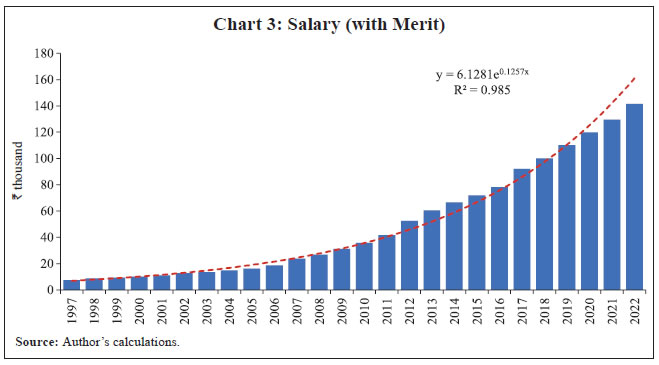

It is important to note that the CAGR of the salary index (with merit) during the 25 year-period from 1997 to 2022 of the stated case is 12.54 per cent. The same without considering merit for the study period is 8.71 per cent. This indicates that 3.52 per cent [100*(1.1254/1.0871)-1] average annual rise in the salary was contributed by merit during the period.

Interestingly, the relative salary of the new recruits who joined on November 01, 1997 and November 01, 2022 was around ₹7.4 thousand and around ₹59.6 thousand, respectively. However, salary of the new recruits, who joined on November 01, 1997, was ₹141.5 thousand (as on November 01, 2022) under the specified assumptions about promotion, etc., as indicated earlier. It may also be noted that the shape of the exponential curve changes significantly in case of merit, which is steeper, as compared to the one without merit (Chart 4).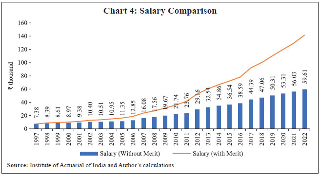

The paper considers a hypothetical cohort of one lakh officers (all aged exactly 27 years as on November 01, 1997), who joined the bank on this date in Scale I. The promotion profile of these officers is assumed to be identical, which was used for constructing the merit salary index. It may be noted that many of these officers may leave the organisation, while some others may die and some may take voluntary retirement before their date of normal retirement (on attaining age of 60 years) viz., October 31, 2030 (same for all in the cohort).

V.1 Multiple Decrements

The paper attempts to estimate these possible exits (either through attrition, or death or early retirement) and remaining through normal retirement. Accordingly, we take three decrements into account in this case, which are (1) Mortality (2) Attrition (including early retirement) and (3) Retirement. The other decrements, such as “ill-health retirement”, are ignored.

Regarding the first decrement of mortality, it is assumed that all officers of the aforementioned cohort follow “Indian Assured Lives Mortality Table 2012-14 Ultimate”.¹² The previous two such life tables were “IALM 1994-96 (Modified) Ultimate” and “IALM 2006-08 Ultimate”, which were effective from January 1, 2005 and April 1, 2013, respectively.

As the life profile of the officers is from 1997 to 2030 (pre-retirement) and 2030 onwards (post-retirement) would impact the pension liability, the latest IALM has been considered in this case. A better approach could be to use all tables with their respective applicable periods. However, this may make the computations more complicated. A comparative study of latest two mortality tables indicates that the mortality profile has changed noticeably at old ages (above 80 years). This underscores the need to use IALM Table 2012-14 for a better reflection of the futuristic mortality of the cohort (Chart 5).

For the second decrement of attrition, it is assumed that the cohort follows an attrition rate as provided in Chart 6. The attrition rate is a crucial input parameter for valuation of such long-term liability, and the rate is unlikely to be smooth.

Our assumption on this rate is based on the fact that the attrition rate should be higher during initial periods of service. Chart 6 exhibits that the attrition rate tapers off since joining over the period of five years from a starting rate of 3 per cent per annum and remains stagnant at 0.5 per cent for about a decade. As quitting before 20 years of service does not result in any payout towards pension under the DB plan, it is disadvantageous for those who quit ahead of 20 years after reaching closer to it. Accordingly, a further tapering off in the rates is assumed till 20 years.

After reaching the point of eligibility for the pension, the attrition results in the eligibility towards pension. Accordingly, the attrition rates beyond this point are indeed the (voluntary/early) retirement rates. It may be mentioned that the attrition rates correspond to “resignations”, while the retirement rates correspond to “early retirement” instead of resignations.

There is a sharp increase in the retirement rate at 20 years of service, which makes an employee eligible to take early retirement. We assume this rate to be at 5 per cent. Again, from this point of time, the retirement rate should show a declining trend, which is reflected in the Chart. After a few years, the rate would dip to its long-run average value of 0.5 per cent.

With the above assumptions on the mortality and attrition rates, an attempt is made to carry out valuation of retirement benefits using the hypothetical cohort, as discussed earlier. For these, both plans (DC and DB) are considered, as both are running simultaneously in the banks. Further, there are some additional benefits, such as gratuity (involving a one-time lump-sum payment) which will typically remain applicable for both the plans and would be linked to the number of years of service and the latest pay drawn ahead of retirement/other forms of exit.

V.2 Demographic and Contribution Functions

We now define some of the actuarial notations as below:

will die before (x+1) years of age

from age x to age x+1 before early retirement age (ERA)

With the given assumptions on mortality and attrition rates, the hypothetical cohort of one lakh officers (all aged exactly 27 years on their joining on November 01, 1997 at the beginning of Scale I) is tracked through the multiple decrement life table. The initial phases are led by exits through quitting (applicable during age 27-46 years) the organisation. A sudden rise in early retirements (applicable during age 47-59 years) is apparent, which tapers off subsequently. It is remarkable to note that the number of deaths of officers increases over the period despite reducing the base each year (Chart 7).

Under the given assumptions, out of one lakh officers, there is an overall attrition of 29,471 officers because of resignations (15,234 cases) and early retirement (14,237 cases). With the expected number of deaths of 8,296, the remaining 62,233 officers (62.2 per cent) shall be expected to retire.

Before constructing various contribution and retirement benefit functions, an attempt is made to compute the actuarial present value (APV) of the payouts towards the salary disbursements of officers, likely to be drawn during the period of service. The APV is a much complex function as compared to the usual present value of certain cash flows (certainty, in terms of known amount and known timing). Indeed, the profile of number of resignations, early retirements and deaths are basic input to the APV. The APV is computed for a series of contingent cash flows, wherein the cashflows depend on some contingent event(s) like death or survival of officer during a period. Accordingly, APV itself is a random variable following a statistical distribution with expected mean of APV and variance of APV.

Using the salary index (with merit) of the gross salary (as derived from Chart 3) and its projected values for future years using a CAGR of 12.50 per cent, round number derived from Assumption 2, as stated earlier, the APV of the aggregate salary is computed for the group/cohort of officers as per the additional assumptions given below:

A constant interest rate of 8 per cent¹⁴ per annum is assumed for the entire period. With this set of assumptions, the APV of the salary is computed and is given in Table 7.

From Table 7, it is observed that the cohort of one lakh officers, who joined in 1997 at an annual gross salary of ₹1 per annum each (total salary ₹1 lakh per annum for the cohort), is expected to result in an APV of around ₹50.98 lakh towards aggregate salary disbursements to the cohort for all the years together. Accordingly, the APV per person is ₹50.98. The annual salary of the last year ahead of retirement (at NRA) is expected to be ₹43.71 (more than 43 times compared to the salary of ₹1 at joining).

In an extreme case, if we assume that all one lakh officers remain in the bank till normal retirement age (i.e., no one quits or takes early retirement or dies), then the APV of the aggregate salary would be around ₹66.08 lakh. In such an extreme scenario, the aggregate salary will be around ₹397.76 lakh (in nominal terms, i.e., without discounting for time value of money). This equates to the APV of the aggregate salary of the cohort under the assumption of interest rate = 0 together with no withdrawal/death etc.

It may be mentioned that many benefits are functions of the pay (could be just basic pay or with add-ons such as special pay, DA etc.). For example, a contribution (say, towards provident fund) could be “y” per cent of the pay. In case, the value of “y” remains the same throughout the period, the contribution functions will be the same whether it is for contribution (PF) or is for the pay itself. Further, the APV of the contributions (say, amounts deposited in the PF) will also be “y” per cent of the APV of the pay. However, withdrawals, such as from PF, at some point(s) of time may complicate the equation, and hence may require necessary adjustments.

V.3 Age Retirement Function

The computations for the retirement benefits are attempted in a similar manner. It may be mentioned that this long-term liability of the organisation is quite different from a DC plan, as covered in Table 7. The nature of this liability is contingent, as no pension is admissible for quitting the job before completing 20 years of service in the organisation. Accordingly, continuing with the same illustration of the characteristics of the cohort, the APV of pension liability is simply ‘zero’ for those who exit from the organisation prior to November 01, 2017 (the assumptions of the hypothetical cohort are taken as the same as in the previous case of demonstration carried out for the contribution function).

The computation of retirement functions requires the life annuity function. The usual annuity (certain annuity) is the present value of a series of future payments for a fixed period at the rate of unit currency of payment per annum. The life annuities are more complicated annuities, which do not have a fixed period and continue till the death of the annuitant.

The pension amount is linked with the basic pay directly, as long as the officer is in service. At the time of retirement (or, early retirement), the initial (starting) pensionable amount is fixed as half of the basic pay plus other applicable pay components, as prevalent just prior to the retirement. However, once this amount is fixed and the officer has already retired, this amount does not track the future basic pay, which will only be available to those who are active in the service. Accordingly, we cannot expect the pension amount to grow with the CAGR of salary (12.50 per cent in our case). After retirement, the pension is largely expected to grow by a rate slightly above the inflation rate, as pension tracks dearness allowance and that is linked with the inflation rate. There will be a minor raise due to subsequent wage revisions though after retirement.

With the above points, the CAGR of pension is assumed to be 7 per cent, which is higher than the observed CAGR of CPI-IW inflation¹⁵ as witnessed during the recent years. Using an interest rate of 8 per cent and pension escalation rate of 7 per cent, a net effective actuarial annual discount rate (v) is computed as 0.9907. Using this net discount rate, the annuity (Case 1) is computed.

A different scenario (Case 2) is also considered. Case 2 pertains to the zero net effective actuarial interest rate, i.e., unit discount rate, v = 1 (assuming same rate of pension growth and interest rate). However, the same (Case 2) is not used in the subsequent calculations. The life annuities are computed for each year of possible retirements (x = 47 to 60 years) and are provided in Chart 8 (details are provided in Table A1 in Annex).

It may be seen that the annuity differentials under these two cases, narrow down consistently with the increase of the age. The annuities are calculated at the end of the year, that is, in arrear.

The retirement functions are now constructed and provided in Table 8. Under the underlying set of assumptions on decrements, out of the one lakh officers who joined the organisation, on an expected term, 8,296 officers will die during their service period, of which, 2,633 will die before age 47 years, so will not be able to take any pension. The remaining, 5,663 will die during age 47-60 years, leading to some applicable pension to their respective families.

Accordingly, a total of 15,234 will be quitting without taking any pension coupled with 2,633 dying without taking any pension. Remaining 82,133 will have either lead to some pension or family pension, of which, 62,233 will survive at least till retirement.

The aggregate pension liability of the cohort is estimated at ₹114.01 lakh as in year 2017 (starting point of pension disbursement). Discounting it back to the time of joining in 1997 gives an estimate of ₹24.46 lakh assuming an interest rate of 8 per cent for discounting. The estimations are based on the rule that the retirees will get pension at half of their pay, which would be applicable at the time of their retirements.

All the computations in this section regarding contribution and retirement functions are carried out to provide expected values of these liabilities and need to be interpreted in actuarial and statistical sense. The estimates are further based on the underlying set of assumptions.

Accordingly, changes in the set of assumptions will lead to corresponding changes in the liability profile of an employer. The computations are complex requiring a lot of assumptions to be made and many other factors may need to be either ignored or approximated.

V.4 DB versus DC Plan – A Comparison

From Tables 7 and 8, the relative cost of pension liability to the employer is assessed. The banks needed to contribute 10 per cent (got revised to 14 per cent in 2021) of the salary towards DC. For the underlying cohort, we computed APV of the aggregate salary as ₹50.98 lakh i.e., ₹50.98 per officer (Table 7). Accordingly, the APV of the contribution would also be 10 per cent for the past years and 14 per cent since 2021. This leads to an expected APV for this cohort to be in the range of ₹5.10 to ₹7.14. In any case, this is substantially lower as compared to the APV of DB pension outgo (Table 8) at ₹24.46. This indicates that the cost of the DB pension plan could be 3 to 5 times higher than that of the cost of DC pension plan under the underlying set of assumptions.

The significantly higher cost of the DB plan to the banks may taper with the passage of time, as the number of employees on the payroll with DB plan would diminish over time and the number of employees with DC plan would rise with the adoption of DC plans by banks.

V.5 Sensitivity of Assumptions - Scenarios

An attempt is made in this section to assess how the APV will deviate from its expected value to align with the revised expected value on account of the corresponding change in the assumptions. The actual realisation on various assumptions could, of course, be quite different from its assumed value. The discussion in the previous section was based on several assumptions. Following this discussion, an attempt is made to assess their marginal impact on liability, which are carried out through scenario analysis.

However, the analysis requires revisiting assumptions regarding (1) Mortality rate (2) Attrition rate (2) Retirement rate (3) Interest rate (4) Inflation rate, and (5) Salary growth rate. Firstly, their marginal impacts on pension liability are considered.

Mortality Rate

The mortality, attrition and retirement rates are the decrements, which do not impact the pension liability directly. Various combinations of these three decrements lead to different composition of the residual cohort at different points of time. The higher decrement rates will squeeze the cohort sooner and vice-versa. Further, a lower/higher rate of one decrement also impacts the loss of life (due to mortality) and exit (due to attrition/early retirement/retirement) together. Indeed, all three are inter-related impacting each other.

As noted, the mortality rates are assumed to follow the “Indian Assured Lives Mortality Table 2012-14 Ultimate”. Although this may be the best available choice for the current study, it may be appreciated that the officers join the organisation after passing through some base level medical checks. Accordingly, their lives, at the time of joining, are not “Ultimate” but rather “Select”. The Select lives are expected to have lower mortality rates than Ultimate lives, especially during the initial years. One way to incorporate it could be through some demographic assumptions. However, no attempt is made for this here. Instead, two different scenarios are taken: the mortality rates at each age are ± 10 per cent (higher/lower) than the earlier assumed rates. That is,

The impact on this change in mortality (keeping all other assumptions unchanged) leads to a different composition of cohort as exhibited in Chart 9.

From the Chart 9, it is observed that the change in mortality will impact the exits as well as early retirements the least. However, it will impact (inversely) the normal retirements with a corresponding change of around ± 1 per cent. The higher mortality leads to lesser number of normal retirements.

The impact of change in mortality on pension liabilities is worked out and is provided in Chart 10. There is a negative association between mortality and APV of pension liabilities. Higher mortality leads to lower APV of the pension liability. Further, the Chart exhibits that a change in mortality by 10 per cent (increase/decrease) translates into a change of around 5 per cent (decrease / increase) in the APV, keeping other factors unchanged.

Attrition and Retirement Rates

The attrition rates are assumed as step functions in this paper (Chart 6). An attempt is made to assess the impact on the cohort profile and the pension liability due to variations in the attrition rates. This is done by changing the assumption of attrition rate as a constant equal to 0.5 per cent per annum (Case 1) and 1 per cent per annum (Case 2) across the entire service period. This way, we assume same decrement rates for “exits” and “early retirements” within each case. Chart 11 shows the cohort profile under the two scenarios along with the earlier assumed variable attrition rates.

It is observed that the assumed attrition rates, varying by age within a wide range of 0.1 per cent to 5.0 per cent per annum across ages have a weighted impact on cohort somewhere in between the two scenarios. Further, the cohort is impacted more significantly than the scenarios of mortality, which was changed by ± 10 per cent (Chart 11).

Now, the impacts are depicted in Chart 12. The two scenarios lead to a change in the APV of liability by +4.32 per cent and -5.00 per cent, respectively. This shows that the existing assumption of varying attrition rate leads to an overall impact somewhere in between a scenario of constant rate of 0.5 per cent per annum and a scenario of 1.0 per cent per annum.

Interest Rate

The assumption of interest rate is the most important assumption, which is used for discounting the future cashflows to the present. The interest rate is assumed to be 8 per cent in the paper. Unlike the decrement rates, the assumption of interest rate does not impact the cohort profile, which solely depends upon various decrement rates alone. The paper computes the stochastic duration¹⁶ of the pension liability. The definition of stochastic duration is similar to traditional duration, wherein the present value (PV) is replaced by APV. Accordingly, it is defined for pension liability as:

Modified Duration = % change in the APV of pension liability / one per cent change in the interest rate.

The modified duration is derived by computing the APV of pension liability at 7.50 and 8.50 per cent interest rates, as the pension liability is expected to have a non-zero convexity.¹⁷ The variation in APV with respect to interest rate is given in Chart 13. The Chart shows inverse relationship between the two, as also seen in the case of traditional duration.

The modified duration is computed as 22.41. This means that the APV changes (decreases/increases) by 22.41 per cent due to a change (increase/decrease) of one per cent point (100 basis points) in the interest rate. From the chart, we see that the APV rises by 11.95 per cent on account of 50 basis points fall in interest rate, but dips by 10.46 per cent when interest rate rises by 50 basis points. Accordingly, the pension liability has a positive convexity, which is common in any DB plan.

Salary Growth Rate and Inflation Rate

The assumption of salary growth rate is yet another important factor in assessing the pension liabilities. For the pension liabilities, the CAGR of 12.50 per cent is assumed. Now, an attempt is made to assess the impact on pension liabilities due to ± 100 basis points change in the CAGR. Thus, the impact on pension liabilities is seen in the two cases, namely where salary growth rate is 13.50 per cent and where it is 11.50 per cent. The assumptions of salary growth rates are applied only to the future years, viz., 2022 onwards. This is because the computed salary scales till 2022 are based on factual data, which need not be modified.¹⁸

Further, the above salary growth rate assumption is applicable only to the active service members. As discussed earlier, the salary growth rate of the inactive service members (pensioners) largely tracks the inflation rates in respective years. Accordingly, two more scenarios have been added, which are pertaining to the inactive lives. It is assumed that the CAGR of pension is 7 per cent in the study. Now, a variation of ± 50 basis points in this growth rate i.e., 7.50 and 6.50 per cent per annum is considered to reflect an inflation rate change by close to 50 basis points either way.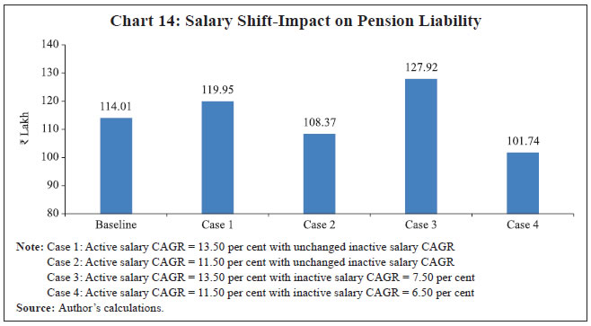

The scenarios of salary growth rates in the pre- and post-retirement phases are provided in Chart 14. From the Chart, it is observed that the assumption of salary growth rate is equally important as that of the interest rate. However, unlike interest rate, the salary growth rate has a positive association with the APV of the pension liability. In other words, a rise in salary will lead to increase in the APV and vice-versa. The APV increases by 5.21 per cent due to 100 basis points increase in pre-retirement salary CAGR (Case 1) and goes up further by 12.20 per cent (combined) due to additional increase in the post-retirement salary CAGR by 50 basis points (Case 3).

Similarly, the APV decreases by 4.95 per cent (Case 2) and 10.76 per cent (Case 4) due to fall in 100 basis points in the pre-retirement salary CAGR with and without 50 basis points fall in post-retirement salary CAGR respectively.

The scenario analysis of key factors in the above paragraphs provides useful insights for assessing the impact of APV of the pension liability. The summary of findings is given in Table 9.

The decrement rates impact the cohort profile, which in turn, impact the APV. The other factors (interest rate, inflation rate and salary escalation rate) do not have any impact on the cohort profile but rather impact the APV directly. The adverse impact is shown in bold in the Table.

V.6 Sensitivity of Assumptions – Worst Scenarios

The impacts, as shown in Table 9, are the marginal impacts, allowing one rate to vary at a time on a ceteris paribus basis. It is very important to consider the joint impacts by allowing all the rates to shift adversely at a time. Some of the rates are positively associated with APV, while others are associated negatively. Two worst scenarios viz., moderate and severe scenarios are considered.

An attempt is made in this section to assess the impact on APV under two stress tests. The relevant rates are allowed to move in adverse directions with two levels (moderate and severe) as shown in Table 10. The adverse marginal impact is assessed. Accordingly, the adverse deviations of assumptions are applied jointly to assess impact of these shocks on liability and covered under the “Stress Tests”.

Two stress tests are applied as below:

• Test 1 - Moderate levels of all factors

• Test 2 – Severe levels of all factors

The impact on APV is exhibited in Chart 15. The APV rises significantly even in the moderate case, which shows the influence of joint impact of many moderate adverse movements occurring together. The APV rises by 25.84 per cent. The severe impact with profound levels of movements in key factors leads to a remarkable 65.63 per cent rise in the APV. The steep rise in the APV under this set of conditions reflects the vulnerability associated with a long-term liability of this kind.

The severe adverse movements of key rates are realistic, although rare. Hence, the possibility of even worse scenarios cannot be ruled out entirely. This is the reason why interest rate and salary CAGR are altered only by about 50-100 basis points. However, actual movements could be even more than this. And yet, a simultaneous adverse movement of all variables may be a rare situation.

The wage revision effective from November 01, 2007, which took place in 2010, may be a good example for illustration. While the wage revision turned out to be higher (17.5 per cent hike) than expected, the upward revision in the gratuity amount (from ₹3.5 lakh to ₹10 lakh), and also the offer of a second option for pension to existing employees and retirees coincided with the wage revision, resulting in huge amount of additional provisioning. This issue was also highlighted by RBI (2011) indicating the systemic concerns arising from this contingent liability.

Section VI
Conclusions and Way Forward

An attempt is made in this paper to construct and project salary indices for the Indian banking sector. The constructed indices fairly represent the Indian banking sector, covering major banks. Accordingly, the indices can be used as an important parameter for macroeconomic analysis. They can also be used as benchmark indices for many other institutions (including non-banking entities like insurance firms and PSUs). Apart from these, the findings may be useful for the financial regulators as well as to the actuarial community, especially for those involved in the pension and retirement benefit plans.

The study finds that the cost of the pension liability to banks under the DB plan could be 3 to 5 times higher than the DC plan, under certain set of assumptions. However, the overall burden of this liability may reduce gradually with the waning of employees in the DB plan and simultaneous increase in the number of employees with the DC plan.

The study also finds that the valuation of the pension liability is very sensitive to the assumption of the interest rate (used for discounting future payouts) and the assumption of future salary escalations. The impact of the interest rate changes on the cost of DB plans could be offset to a large extent by making liability driven investments (LDIs) in order to create matching assets subject to its availability.

The findings from the paper are expected to be useful for various HR-related policy decisions, such as, review of employers’ long-term liabilities, committed wage revisions, terms of promotion, optimisation of demographic profile of officers, etc. The organisations may use these indices and assess the impact of such liabilities on their balance sheet within the overall framework of enterprise risk management. The degree of sensitivity to various actuarial assumptions of the pension liability as quantified in the paper is useful in identifying and assessing the role of these assumptions, which might be crucial in the overall valuation exercise of such contingent liabilities of the organisation.

The paper also opens up wide possibilities for future studies on this subject. For example, probability distribution of APV of pension liabilities as an output to the various input variables can be carried out using a Monte Carlo Simulation method as an extension to this stress test. This could be facilitated by the availability of the actuarial computing software.

References

Dadlani, D. & Jain, K. (2022). Sensitising to Sensitivities, 5th TechTalk in Employee Benefits, Institute of Actuaries of India, June.

European Commission (2011). The 2012 Ageing Report: Underlying assumptions and projection methodologies, European Economy, No. 4.

Franzen, D. (2010). Managing investment risk in defined benefit pension funds, OECD Working Papers on Insurance and Private Pensions, No. 38.

Formulae and Tables for Examinations (2002). The Faculty and Institute of Actuaries, United Kingdom.

Gingrich, E. (2015). US Retirement Market and the Role of the Actuary. Paper presented at the 17th Global Conference of Actuaries (GCA), Mumbai, February.

IBA (2015). Dearness Allowance Time-series Quarterly Rates, Indian Banks’ Association.

IMF (2004). Market Developments and Issues, Global Financial Stability Report, September.

IMF (2017). Getting the Policy Mix Right, Global Financial Stability Report, April.

Kumar, V. (2013). Understanding trends in salary escalation rates in private sector, Research Project, Institute of Actuaries of India, Mumbai.

Kumar, V. (2014). Research Projects – Takeaways, A Presentation at the 10th Seminar on Current Issues in Retirement Benefits (CILA), Institute of Actuaries of India, September.

Saha, M. (2013). “RBI wants all PSBs to have uniform pension provision”. Business Standard: http://www.business-standard.com/article/finance/rbi-wants-all-psbs-to-have-uniform-pension-provision-111071400059_1.html

Pandit, D. K. (2014). Employees Benefits and Actuarial Advice. Paper presented at the 16th Global Conference of Actuaries (GCA), Mumbai, February.

Pandit, J. D. & Kandoi, K. (2021). Actuarial Valuation of Employee Benefit – Impact of Social Security Code and COVID-19, A Presentation at the Western India Regional Council (WIRC) of the Institute of Chartered Accountants of India (ICAI), April.

Patel, Urjit R. (1997). Aspects of Pension Fund Reform: Lessons for India, Economic and Political Weekly, September, pp-2395-2402.

Peethambaran A. P. (2014). A Model (Deterministic) for Leave Benefit Valuation, Paper presented at the 16th Global Conference of Actuaries (GCA), Mumbai, February.

Ramaswamy, S. (2012). The sustainability of pension schemes, BIS Working Paper, No. 368, Monetary and Economic Department, Bank for International Settlement, Basel.

RBI (2011). Financial Stability Report, Reserve Bank of India, June issue (Box.3.2).

Sriram, K. (2014). Developing Appropriate Investment Strategies for Funded Employee Benefit Plans – Need & Scope for Actuarial Involvement. Paper presented at the 16th Global Conference of Actuaries (GCA), Mumbai, February.

Sriram, K. & Patel, K (2020). Sustainable Retirement for All. Paper presented at the 21st Global Conference of Actuaries (GCA), Mumbai, February.

Annex

^* R K Sinha (rajatsinha@rbi.org.in) is Director in the Monetary Policy Department (MPD), Reserve Bank of India. The author gratefully acknowledges the comments received from an anonymous reviewer, and also to Ranjeev, Assistant Adviser, Department of Statistics and Information Management (DSIM), who discussed the paper and offered his comments in the Department of Economic and Policy Research (DEPR) Study Circle Seminar. The author sincerely thanks officials of DSIM for their suggestions in earlier versions of the paper. The author is also thankful to Pallavi Chavan and her team in Development Research Group (DRG), DEPR for their valuable suggestions. The views expressed in the paper are those of the author and do not represent the views of the Reserve Bank of India.

¹ The position is defined for a certain designation / grade with certain number of years of experience. The position of an employee changes every year with added number of years of experience and/or due to periodic promotion to the next grade.

² The Consumer Price Index for the Industrial Workers (CPI-IW) is considered by most of the employers in India to compile the dearness allowance (DA), which is incorporated to reflect the inflationary rise in the salary.

³ At present, these banks have possibly outsourced the valuation of their contingent liability to some actuarial firms, which would have internally developed suitable salary indices for the necessary valuations.

⁴ The Institute of Actuaries of India has increasingly engaged in conducting various seminars such as “Capacity Building Seminar on Retirement Benefits”, “Webinar on Retirement Benefits”, “Global Conference of Actuaries”, “India Fellowship Seminar”, etc. The links for presentations/papers are available on its website (https://www.actuariesindia.org) covering updates on the subject including regulatory developments.

⁵ The Officers’ cadre covers seven scales, namely, Scale I (lowest cadre) through Scale VII (highest cadre).

⁶ The Bipartite on the “Conclusion of discussions between Indian Banks’ Association and Workmen Unions” deals with wage settlements for the staff of the banks. The latest Bipartite settlement is the 11th, in series, which was signed on November 11, 2020.

⁷ The Joint Note on the “Conclusion of Discussions between Indian Banks’ Association and Officers’ Association” was also signed on November 11, 2020. The note provides various details and recommendations relating to the wage revisions applicable to a specified list of banks, wherein the wage revisions in the officer’s cadre would be followed.

⁸ The paper considers basic pay, dearness allowance (DA), special allowance and city compensatory allowance (CCA) for the gross salary. Accordingly, other components of salary such as house rent allowance (HRA), fixed pay allowance (FPA), stagnation allowance, qualification allowances etc. are not considered, as they are largely specific to a particular cohort of employees. For example, the HRA is applicable only to those, who do not reside in banks’ quarters, or qualification allowance is only applicable to those, who procure certain qualifications like Ph.D. or Certified Associate of Indian Institute of Bankers (CAIIB) etc.

⁹ The rise in the dearness allowance was largely non-linear till January 31, 2005, as the slabs for DA were not used to be neutralised till that time across the Cadres. The 100 per cent neutralization was effective w.e.f. February 01, 2005, which resulted in higher degree of linearity between the DA and CPI-IW.

¹⁰ The paper focuses on the pension liability although other liabilities such as gratuity, leave encashment, medical assistance, etc. are also linked with salary indices and thus could be analysed in a similar way.

¹¹ In the absence of historical data on promotion timings, the assumption of promotions at every seven years is made to reflect a generic realistic scenario (four promotions in a service life of 28-30 years, although they may not be equally spaced).

¹² This mortality table is the latest published life table, published by the Institute of Actuaries of India (IAI) with concurrence of the Insurance Regulatory and Development Authority of India (IRDAI) and is effective from April 01, 2019. The paper considers this mortality table to reflect the future likely survival rates of the officers of the banks in a better manner.

¹³ The attrition rate for the public sector banks was assessed to be at around 0.50 per cent, as per Saha (2013). The rate for the private and foreign banks are likely to differ from this average and is likely to be on an upper side. The sensitivity of different attrition rate assumptions is analysed in the latter part of the paper, which provide possible impact and implications on the pension liability.

¹⁴ A constant interest rate of 8 per cent is assumed for the study because of the nature of liability, which is a long-term. Accordingly, a baseline assumption is made and sensitivity is assessed if we depart from this baseline.

¹⁵ The CAGR of CPI-IW inflation rate was slightly below 7 per cent during 15 years (2001-16) at the base year 2001, and dipped to around 4.4 per cent during the subsequent 6 years (2016-22) at the base year 2016.

¹⁶ Stochastic duration is different and more complex from the traditional duration of fixed income, wherein cashflows are certain with regard to their timings and amount. Stochastic duration is based on uncertain cashflows, which depends on some contingent events.

¹⁷ The non-zero convexity results when the duration is not a constant and itself changes with the level of interest rates. The convexity is the derivative of duration of pension liability with respect to interest rate. The convex (positive) nature of convexity can be depicted from Chart 13, which is usual in long-term bonds also.

¹⁸ This is unlike other assumptions, such as, various decrement rates, which are applied during entire period. However, there are not known to the researcher.