Sujeesh Kumar, Pawan Kumar and Anand Prakash* Received on: January 18, 2022
Accepted on: June 17, 2022 This paper examines the nature and degree of causal relationship between credit, investment and business cycles in India during the period 1950-51 to 2020-21. The duration of cycles and their turning points have been estimated using the National Bureau of Economic Research (NBER) dating procedure. The phase synchronisation of cycles is assessed using a concordance index. The paper finds that the credit, investment and business cycles interact with each other and have bi-directional causal linkages. The results also indicate an increase in phase synchronisation of the Indian credit cycle with that of the emerging market economies (EMEs) and advanced economies (AEs) after the global financial crisis. JEL Classification: C22, E32, E58, D91 Keywords: Credit cycle, business cycle, investment cycle, synchronisation, concordance index, non-bank sources Introduction Studies on the cyclical patterns of macroeconomic variables are not new, and the cyclical pattern analysis indeed has its own history (Tinbergen, 1939; Schumpeter, 1954; Lee, 1955). A significant development in the field of economic cycles was the identification of cycles and their phases, such as expansion, crisis, recession and recovery (Kitchin,1923; Schumpeter, 1954; Lee,1955). Although this was the initial work, the focus of cyclical pattern analysis even now is centered on these aspects. There have been instances where the economic cycles have been named after the inventors, such as the ‘Juglar cycle’ for fixed investment and the ‘Kuznets swing’ for infrastructure investment, among others (Korotayev et al., 2010). The cyclical patterns of key macroeconomic variables and their behaviour have fascinated researchers, and as a result, various theories around these cycles have been propounded in the literature. Historically, the emphasis was given on the business cycle as it dealt with the growth aspects of an economy. The business cycles were extensively studied across the globe, including in the Indian context. However, after the global financial crisis (GFC) in 2008, the focus has shifted towards financial cycles, notwithstanding the continued importance of the business cycle analysis. The GFC has kindled greater interest among economists in the cyclical behaviour of financial variables. This aspect has also engaged the attention of researchers and policymakers, including central bankers, all over the world. The recent literature suggests that financial cycles duration is larger than that of business cycles. This pattern has been witnessed across the globe, especially after the GFC (Claessens et al., 2011, 2012; Drehmann et al., 2012; Strohsal, 2015; Pontines, 2017; Borio et al., 2018). The financial cycle analysis generally involves financial variables, such as bank credit, housing prices, non-bank credit, equity prices, etc. The literature on financial cycles for the developed markets is vast. However, the studies for the emerging market economies (EMEs) are relatively few, specifically in the Indian context. The literature for India shows that business cycles have got elongated after the introduction of economic reforms during 1990-91. In the Indian context, there are a few studies on the business cycles as well (Mall, 1999; Mohanty et al., 2003; Dua and Banerji, 2006; Dua and Banerji, 2012; Ghate et al., 2013; Pandey et al., 2017). Some studies in the Indian context have also examined the duration of the investment cycle. The investment cycle should ideally be aligned with the business cycle, as investment and GDP growth are closely related. A recent study has suggested that investment cycles in India have an average duration of three years (Raj et al., 2018). A study on the financial cycle in the Indian context was first attempted by Behera and Sharma (2019), which concluded that the financial cycle has a longer duration than that of the business cycle. Specifically, they found that the average duration of business cycles in India was about five years and that of the credit cycle about 15 years in the post-reforms period. The financial cycle analysis focuses on the aggregate effect of all financial variables on the real economic variables. Even though credit is one of the main components of a financial cycle, a separate and detailed analysis of credit cycles is not available in the Indian context. Credit cycle is not only crucial in connection with the financial cycle analysis but also for the study of financial stability. As a result, credit cycles have engaged the attention of central bankers, given their mandate of financial stability. Credit is also associated with the business and investment cycles. The co-movement between credit and business cycles reflects the relationship between financial and real sectors of the economy. Financial frictions can amplify credit cycles, resulting in their longer durations and amplitudes. Several studies have argued that financial development beyond a threshold level may inhibit growth, specifically excess credit growth may cause reversal of the economic growth process (Cecchetti and Kharroubi, 2012; Law and Singh, 2014; Rath and Kumar, 2021). Therefore, studying credit booms and credit crunches is important, especially after the GFC. Generally, economists analyse the boom and bust phases of an economy through cycles of various macroeconomic variables, such as output, investment, consumption and credit. The term ‘economic cycle’ refers to economy-wide fluctuations, that occur around a long-term growth trend, in production or economic activity over several months or years. Besides, these fluctuations involve alternate shifts over time between periods of relatively rapid economic growth (expansion or boom), and periods of stagnation or decline in growth (recession or depression) (Sullivan and Sheffrin, 2006). The cyclical patterns or fluctuations can be visible over longer periods of time for any macroeconomic variables. In the conventional cyclical analysis, cycles of macroeconomic variables, such as credit, investment and GDP are estimated using long time-series data and applying a suitable extraction methodology. These cycles interact with each other as the macroeconomic variables are closely inter-related. In the financial systems, funds are raised from either banks or non-bank sources. The non-bank sources of finance are generally heterogeneous and include private placements of debt instruments, public offerings or loans from a varied group of lenders like investment funds, external borrowings from foreign lenders, etc. The non-bank credit in AEs is relatively larger than EMEs. However, the dependence on non-bank sources has been growing even in EMEs in the recent years, with non-bank sources increasingly complementing bank credit. The synchronisation of the bank credit cycle and non–bank credit cycle is not uniform and can vary from country to country or can change due to financial shocks in the economy. Studies have also shown that excessive growth of bank credit is a leading indicator of systemic banking crises. Non-bank credit cycle can act as a leading indicator of currency crises or sovereign debt crises (Kemp et al., 2018). Yet, given the growing importance of non-bank funds, it is important to assess the association between bank credit and non-bank funding cycles. Against this backdrop, this study examines the behaviour of the credit cycle, both bank credit and non-bank funds, investment cycle, and business cycle in India during the period 1950-51 to 2020-21. The study analyses the phase synchronisation between credit, investment and business cycles. This study also analyses the synchronisation between credit cycle of India with that in EMEs and AEs. The remaining part of the paper is structured as follows: Section II presents a brief review of literature. Section III presents the stylised facts and Section IV discusses the key non-bank sources of finance in India. Section V discusses the methodology and data used in this paper. Section VI explains the empirical findings, while section VII presents the concluding remarks. Section II
Review of Literature Finance was generally viewed as a sideshow to macroeconomic fluctuations as part of the pre-GFC paradigms, but this view was proved wrong during the GFC (Drehmann et al., 2012). After the GFC, there has been an increased interest in studying the relationship between real and financial variables. Traditionally, studies about business cycles have focused on the behaviour of real macroeconomic variables. Cycles of financial variables attained importance particularly after the GFC. Furthermore, longer durations of financial cycles were observed after the GFC. The idea of a long financial swing was initially discussed by Minsky (1964). Credit plays a prominent role in the financial development of any economy. The credit cycle is distinct from the business cycle in its frequency and amplitude (Aikman et al., 2015; Drehmann et al., 2012). Credit cycle has the predictive ability, as it can act as a leading or a lagging indicator of economic growth. Some studies assert that credit is a lagging indicator (Haavio, 2012; Haavio et al., 2013; Runstler and Vlekke, 2017), while others claim it to be a leading indicator (Gomez-Gonzales et al., 2014) of business cycles. In addition to the credit cycle, recent studies have also dealt with the financial cycle, with credit as one of its key components. For the construction of a financial cycle, researchers have typically considered variables such as bank credit, other forms of credit, housing prices, etc. The financial cycle is used to analyse financial stability by central banks. Borio et al. (2018) studied financial cycles extensively and their implications for the economy, particularly in connection with the GFC. Empirical research suggests that financial cycles have a longer duration and shorter frequency than the business cycle (Claessens et al., 2011, 2012; Drehmann et al., 2012; Strohsal, 2015; Pontines, V., 2017; Borio et al., 2018). Based on a large country sample covering 40 years, Borio et al. (2018) noted that credit booms undermine growth, as they result in the misallocation of resources to a sector with lower productivity growth, and the subsequent impact will be larger if the boom is followed by a banking crisis. Hieberta et al. (2018) empirically examined the characteristics of financial and business cycles of 13 European Union countries. They found that financial cycles have a longer duration and greater symmetry than business cycles. Moreover, among the 13 countries, those which experienced severe financial downturns exhibited a weaker similarity in the patterns of their cycles. This showed that financial cycles cannot be similar for countries that have experienced financial crises. Alternatively, the crises could be impacting financial cycles differently depending on their severity and the individual country’s economic scenario and policy actions. Runstler and Vlekke (2017) studied the cyclical components in GDP, credit volumes, and house prices for the US and the five largest European economies. Their estimates suggested that large and long cycles of credit and house prices were correlated with a medium‐term component in GDP cycles. Credit can also be raised from non-bank sources. Oftentimes, a non-bank form of credit is a substitute for bank credit if the bank credit is costlier or not easily available for the investors (Kemp et al., 2018). IMF (2015) refers to market‐based financing as a ‘spare tyre’ during the periods of constrained bank credit. The literature suggests that a large reliance on non-bank debt or market-based finance, relative to bank credit, can facilitate economic growth and financial stability (Gambacorta et al., 2014; Bats and Houben, 2017). On the other hand, there are several examples of stress events in the non‐bank sector, and some of which have been systemic in nature (ESRB, 2016). The main focus of credit cycle analysis is to explain either the economic growth or financial stability. There are a few studies that connect credit cycle to the monetary policy as well. According to the findings of Brauning and Ivashina (2019), during the monetary policy easing cycles in the US, the volume of loans sanctioned by foreign banks increased significantly in the EMEs. This was followed by credit contraction when the monetary policy was tightened by the US. Thus, the US monetary policy influenced credit cycles in EMEs, as the availability of foreign bank credit to EMEs is closely related to the US monetary policy. Credit growth facilitates investment and economic growth, and higher economic growth in turn leads to more demand for investment and credit. Thus, credit has causal relationships with both investment and GDP. As noted by Kent and D’Arcy (2001), the strength of economic activity determines credit demand, and the financial system’s health influences credit supply, which in turn affects the economic activity. Episodes of rapid credit growth (i.e., credit booms) have also been associated with periods of economic distress owing to overheating of the economy (Mendoza and Terrones, 2008). Therefore, excessive credit growth is one of the critical early warning indicators of macroeconomic and financial instability in an economy. Credit cycles may often develop as a result of the business cycle, as banks’ lending typically accelerates during a period of economic expansion and weakens during a contraction phase. From the supply side, during economic booms, business optimism and rising collateral values1 lead bankers to expand lending even at the cost of loosening lending standards. By contrast, during downturns, a pessimistic outlook results in deferred lending decisions (Samantaraya, 2007 and Ariccia et al., 2012). From the demand side, inherent optimism (pessimism) about economic activity, connected with the business cycle, expands (restricts) investment and consumption spending in response to higher (weaker) expected income, wealth, and effective demand, influencing credit demand. Additionally, during the expansionary phases, abundant credit supply leads to higher investment and consumption, and enhanced collateral values. The process is reversed during a downturn. This implies that the nature of bank credit is typically procyclical (IMF, 2008). Banerjee (2011) also noted the procyclical nature of credit in the Indian context. Procyclicality of the financial system generally refers to the mutually reinforcing interactions (‘positive feedback’) between the real and financial sectors of the economy that amplify the business cycle and are usually the source of financial instability (Drehmann et al., 2011). This procyclicality of credit has been a major driver of the increase in the amplitudes of business cycles, in effect, exacerbating the economic cycles (Banerjee, 2011). Therefore, it is vital to understand the cyclical characteristics of credit and its relationship with other major macroeconomic variables, while formulating early warning indicators of macroeconomic imbalances and devising policy response to business cycles. Section III
Stylised Facts III.1. Characteristics of Credit, Investment and Business Cycles in India As noted earlier, the relation between real and financial sectors have attracted greater attention of researchers and policymakers after the GFC. In a strong bank-based economy like India, bank credit is a major source of finance. Bank credit has also supported infrastructure financing in recent decades. The investments in physical assets get reflected in the gross fixed capital formation (GFCF), which is one of the major components of GDP. The 3-year moving averages of GDP, investment, and bank credit growth rates (y-o-y) are presented in Chart 1, which shows that acceleration or deceleration in growth rates of these three variables are closely associated with each other. Bank credit growth, which touched its peak in 2006-07, has witnessed a downtrend since the GFC, which coincided with a slowdown in investment and economic growth. 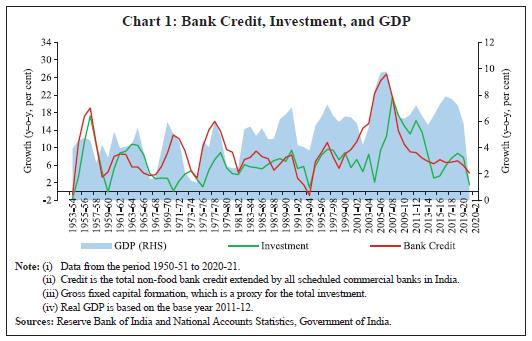
| Table 1: Summary of Key Growth Statistics | | Periods | Growth (per cent) | Volatility | | Bank Credit | Invest-ment | GDP | Bank Credit | Invest-ment | GDP | | 1950-51 to 1979-80 | 7.9 | 4.9 | 3.6 | 8.3 | 7.0 | 3.3 | | 1980-81 to 1989-90 | 7.6 | 6.2 | 5.6 | 2.9 | 1.8 | 1.9 | | 1990-91 to 2007-08 | 11.9 | 8.0 | 6.4 | 10.0 | 8.7 | 2.7 | | 2008-09 to 2020-21 | 6.5 | 6.8 | 5.5 | 2.7 | 7.4 | 4.1 | Note: GDP, investment, and credit growth are in real terms. Volatility measured by the standard deviation.
Sources: Reserve Bank of India and National Accounts Statistics, Government of India. | Some of the key growth statistics of the Indian economy over different time periods are given in Table 1. The period between 1950-51 to 2020-21 is split into four sub-periods: 1950-51 to 1979-80, 1980-81 to 1989-90, 1990-91 to 2007-08 and 2008-09 to 2020-21. During the first three decades after independence (1950-51 to 1979-80), the annual average economic growth rate was the lowest at around 3.6 per cent. During this period, average growth rates of investment and credit were 4.9 per cent and 7.9 per cent, respectively. However, the Indian economy experienced a turnaround in the 1980s, with a slow shift towards liberalisation, as GDP and investment growth rate picked up significantly, even though credit growth softened marginally. In the 1990s, the initiation of economic reforms in the early 1990s brought about structural changes in the economy. Though, credit growth decelerated somewhat in the 1990s, it subsequently recovered sharply, registering a double-digit growth from the beginning of the 2000s that continued till the advent of the GFC in 2007-08. GDP and investment growth registered an increase during the period 1990-91 to 2007-08. However, during 2008-09 to 2020-21, the average growth of all the above-mentioned macro variables moderated significantly. The pace of credit growth, which was 2.2 times and 1.6 times that of GDP and investment growth, respectively, during 1950-51 to 1979-80, moderated to 1.4 times and 1.2 times during 1980-81 to 1989-90. During the period 1990-91 to 2007-08, credit growth was 1.9 times and 1.5 times that of GDP and investment growth, respectively. However, the volatility of GDP, investment, and credit growth, which was relatively low during the 1980s, increased significantly in this phase. In the post-GFC period, during 2008-09 to 2020-21, credit growth reduced noticeably. In this period, volatility in investment and credit growth rates moderated, though volatility in GDP growth increased. Section IV
Sources of Non-Bank Finance in India Even though the financial requirements of the Indian economy are primarily met by the banking sector, alternative non-banking sources are increasingly being used for financing investment projects. For instance, the Indian corporate sector relies on external commercial borrowings (ECBs) and funds mobilised from the capital markets, mainly equities and private placements of bonds. Moreover, new avenues, such as venture capital funds, private equity funds, and angel funds are being used, particularly by start-ups. Research on alternative investments in EMEs is at a nascent stage but is growing rapidly (Cumming and Zhang, 2016). In this study, for the construction of the non-bank2 funding cycle, aggregate value of three sources of non-bank finance viz., (a) external commercial borrowings (ECBs), (b) resources mobilised from capital markets, and (c) foreign direct investment (FDI) have been used. IV.1 External Commercial Borrowings The borrowing behaviour of Indian corporates is broadly driven by the investment demand, which, in turn, is a function of expected economic growth in the future. The investment demand can be financed through external funds or internal funds. ECBs are one of the sources for meeting such fund requirements and have emerged as a significant source of the flow of funds in India (Chart 2a). A firm’s preference between borrowings from the domestic capital market or the overseas markets is typically made after a thorough long-term financial planning (World Bank, 2007). IV.2 Foreign Direct Investment in India Following liberalisation in 1991 and the subsequent amendment of the new industrial policy (NIP) coupled with integration of the Indian economy with the world economy, the industrial policy regime has changed significantly. The policy reforms have enhanced the attractiveness of India as a long-term investment destination resulting in a significant increase in FDI flows. Foreign investors come to India also for its locational advantages, relaxed entry norms, and growing interest in the country’s services and manufacturing sector. Consequently, FDI inflows into India have increased significantly over the last decade (Chart 2b). IV.3 Resources Mobilised through Primary Markets Resource mobilisation through primary markets covers the Initial Public Offerings (IPOs) and private placements. The quantum of private placements has witnessed a significant increase in recent years over public issues (Charts 2c and 2d). Section V
Methodology and Data Representing an economic or financial time series variable by Yt, a cycle yt can be defined as a pattern seen in the series. Burns & Mitchell (1946) have defined business cycle as a type of fluctuation in the aggregate economic activity of nations. Thus, the cyclical characteristics of cycle yt are extracted from the corresponding time series data of variable Yt. The nature of yt is generally described with parametric statistic models that would effectively describe the temporal behaviour of yt. In the cyclical analysis, the first step is to extract the cyclical component of the time series Yt, after adjusting the seasonal fluctuations in Yt, using a suitable methodology. There are three common approaches to estimate cycles. The classical approach3, the growth cycle approach, and the growth rate approach. In the Indian context, especially in the post-reforms period, the most suitable approach is the growth cycle or growth rate cycle approach, as the classical approach is not useful in identifying the turning points (Patnaik and Sharma, 2002; Mohanty et al., 2003; Dua and Banerji, 2012; Pandey et al., 2017). Following Pandey et al. (2017), the growth cycle approach has been used for the estimation of cycles in this paper. Further, the estimation of any cycle is accomplished by identifying the turning points in yt, i.e., peaks and troughs. The turning point dates mark the beginning of expansion and contraction phases of an extracted cycle yt. There are various filters commonly used for extracting cyclical components of a time series. Each one has its own advantages and disadvantages depending upon the algorithms used. Popular among them are Hodrick - Prescott (HP) filter, Band-Pass (BP) Filter, Hamilton filter, and Christiano – Fitzgerald (CF) filter (Christiano and Fitzgerald, 2003). One of the limitations of the HP filter is that the cycle estimated using HP filter is sensitive to different values of the smoothing parameter (Bjornland, 2000). The choice of the smoothing parameter (λ) in the HP filter has implications for the variability of the trend term. Further, it can yield spurious relations that are unrelated to the underlying data-generating process (Hamilton, 2016). Therefore, alternate filters have been used in the literature for extracting the cyclical components. One of most effective filters is the CF filter, which has been used in this paper. This filter is time-invariant and works based on the power spectrum of the time series. It does not change the relation between time series components at any frequency. These are the advantages of the CF filter over other filters, such as the HP filter or BP filter. Bry and Boschan (1971) first gave the dating algorithm (BB) for the estimation of turning points, which is based on the cyclical components extracted from the time series. This extraction technique can be applied to a monthly or quarterly data series. The quarterly version of the BB algorithm can also be combined with some censoring rules, sometimes called Bry and Boschan Quarterly (BBQ)4 algorithm. A popular dating procedure is the NBER procedure, which is based on the BB algorithm. This study uses the NEBR dating procedure to obtain the turning points, durations, and amplitude of the cycles. Conventionally, business cycle analysis deals with a period of 2-8 years, referred to as short cycles in the business cycle literature and cycles covering a period beyond eight years are generally referred to as medium cycles. In this paper, both short cycles and medium cycles of all variables have been estimated for a better understanding of the behaviour of the cycles and the relationship between them. Using the above equations (1) and (2), a measure of the degree of synchronisation between the cycles, called the concordance index (CI), proposed by Harding and Pagan (2002) is calculated as follows: CI indicates the number of periods for which the two cycles are in same phase and averages them out over T periods. The values of CI can range from zero to one with zero indicating perfect misalignment between phases of two series considered and one implying perfect alignment. Various steps are involved starting from the estimation of the cycle to the calculation of the concordance index as follows: i) First, we seasonally adjust the quarterly data series for seasonal fluctuations. In India, the official statistics do not feature seasonal adjustment. Therefore, the series is seasonally adjusted using the X-14-ARIMA method. ii) In the second step, the cyclical component of each series is extracted from the seasonally adjusted log transferred series using Christiano-Fitzgerald asymmetric filter. iii) Next, the turning points and durations of the cycles are estimated using the NEBR dating procedure. The details of the NEBR procedure and CF Filter are given in the Annex A1 and A2. iv) Finally, the phase synchronisation between various cycles is estimated using a concordance index. The four key variables used in the paper are bank credit, non-bank funds, investment, and GDP. Bank credit is the total non-food credit extended by all scheduled commercial banks in India. Non-bank funds refer to alternative sources of funding for the Indian corporates, such as external commercial borrowings (ECBs), resources mobilised from primary markets, which include public offerings and private placements, and foreign direct investment (FDI). To estimate the business cycle, total output of the country measured by real GDP has been used. The gross fixed capital formation, which is a proxy for the total investment, has been used to derive the investment cycle. Annual time-series data have been used for extracting GDP, investment, and bank credit cycles. However, non-bank funding cycle has been derived from quarterly data, as annual data are not unavailable over a longer period. Quarterly GDP, investment, and bank credit data have also been used to estimate cycles in order to compare their synchronisation with the non-bank funding cycle. All variables are in real terms and quarterly data are seasonally adjusted using the X-14-ARIMA method before estimating the cycles. Annual series are for the period 1950-51 to 2020-21, while quarterly series are for the period quarter ending June 1997 (1997-98: Q1) to the quarter ending March 2020 (2019-20: Q4). The details of each variable and their sources along with descriptive statistics are given in Annex Tables A3 and A4. Section VI
Empirical Analysis VI.1. Cycles and Turning Points The severity of the depression phase of a cycle or the strength of its expansionary phase is measured by the duration and amplitude of the cycle. Duration measures the length of a cycle, whereas amplitude measures the degree of change in the cyclical phase. A downturn’s duration can be computed by calculating the number of years/quarters between a peak and a trough, while an upturn’s duration can be determined by counting the years/quarters that pass from trough to peak. The amplitude for the downturn is computed based on the deceleration in each respective variable from the peak to the next trough, while the same for the upturn measures the change in a variable from trough to peak. The cyclical components of bank credit, investment and GDP for the period 1950-51 to 2020-21 have been extracted using the CF filter and turning points are identified by the NEBR dating procedure. The credit cycle, investment cycle and the business cycle (GDP cycle) have been plotted in Chart 3. The cycle turning points have been analysed with reference to the reforms period in India, as macro analysis typically compares post-reforms and pre-reforms periods (Ghate et al., 2013; Banerjee, 2011; Behera and Sharma, 2019). Accordingly, the business, investment and credit cycles have been separately analysed for two periods – from 1950-51 to 1990-91 (the pre-reforms period) and from 1991-92 to 2020-21 (the post-reforms period). The basic cyclical characteristics of these macroeconomic variables are given in Table 2. As indicated earlier, the descriptive statistics of the cyclical characteristics are also given for pre- and post-reforms periods. Volatility measured by the standard deviation of each cyclical series is similar across short cycles, while medium cycles of GDP and credit exhibit higher volatility in the post-reforms period as compared to the pre-reforms period. However, the investment cycle exhibited lower volatility in the post-reforms period. The relative volatility5 of medium duration credit cycle was higher than that of an investment cycle during both the pre- and post-reforms period, while it was smaller for the short cycle in the post-reforms period. In general, the contemporaneous correlations of both credit and investment cycles with the GDP cycle increased during the post-reforms period. VI.2. Durations of Cycles Estimates of the duration of expansionary and contractionary phases of the Indian business cycles are presented in Table 3. According to our analysis based on short cycles, the duration of both the investment and business cycles is eight years, while the duration of the credit cycle is seven years. Considering medium cycles, the average duration of the credit cycle in both expansion and contraction phases is longer than that of the business cycle. The average duration of the credit cycle is 17 years, while that of the business cycle is nine years. The duration of the expansion phase of the credit cycle varied from 5 to 10 years, while the duration of the contraction phase varies from 3 to 14 years (Annex Tables A5 and A6). The presence of large credit cycles was observed after the initiation of financial sector reforms in India. Behera and Sharma (2019) also noted the presence of medium-term financial cycles in India in the post-reforms period. | Table 2: Cycle Statistics for the Indian Economy Based on Annual Data | | | Pre-reforms (1980-81 to 1989-90) | Post-reforms (1990-1991 to 2020-21) | | Mean | Volatility | Relative Volatility | Correlation | Mean | Volatility | Relative Volatility | Correlation | | Short Cycle | | | | | | | | | | GDP | -0.0002 | 0.02 | 1 | 1 | 0.0002 | 0.02 | 1 | 1 | | Investment | -0.0002 | 0.04 | 1.96 | 0.32 | 0.0015 | 0.04 | 2.15 | 0.80 | | Credit | -0.0005 | 0.05 | 2.39 | 0.50 | 0.0006 | 0.03 | 1.51 | 0.57 | | Medium Cycle | | | | | | | | | | GDP | 0.0004 | 0.01 | 1 | 1 | 0.0055 | 0.03 | 1 | 1 | | Investment | -0.0027 | 0.06 | 4.45 | 0.54 | -0.0013 | 0.04 | 1.41 | 0.60 | | Credit | 0.0142 | 0.08 | 5.75 | 0.19 | -0.0127 | 0.13 | 4.42 | 0.13 | Note: (i) Volatility is measured as the standard deviation of the variable of interest and it gives the aggregate fluctuations of the variable.
(ii) Correlation is the simple Pearson correlation between the variables and GDP.
Source: Authors’ estimates. | The average duration of the credit cycle tended to be longer than the duration of the business cycle, as any deterioration in corporate fundamentals or asset prices takes time to manifest and financial vulnerabilities reduce over a long-time horizon as balance sheet repair is a protracted process, thereby leading to an elongation of the duration of credit cycle. The difference in length of the cycles means that the span of one credit cycle is longer than one business cycle. This implies that even when business activities slow down, there may be a chance of over-extension of credit leading to the build-up of asset price bubbles. The reverse may happen when economic activities start picking up but a pickup in credit offtake may be delayed. Thus, there may be leads and lags resulting in a credit cycle duration being longer than that of a business cycle. Any failure to recognise the longer duration of credit cycle may result in greater economic disruption, especially when the asset price bubble created by excessive credit extension bursts. During periods of uncertainty, there could be time and cost overruns, which may extend the length of the credit cycle, as banks may continue to lend, even at a slower pace, due to the effect of monetary or macro-prudential policies used by the authorities to address the situation. Similarly, the duration of expansionary and contractionary phases of a credit cycle is not expected to be symmetric over time; various macro-economic, financial, and other shocks may prolong/shorten the duration of a phase of a cycle. The duration of the business cycle varies in the range of 3 to 6 years and 3 to 7 years in the expansionary and contractionary phases, respectively. It is observed that the contractionary phase of the credit cycle is more prolonged than the expansionary phase. The average duration of contractionary phase of the credit cycle is around 11 years, which is higher than the average duration of around seven years in the case of an expansionary phase. The prolonged contractionary phase of the credit cycle witnessed in the post-GFC period may be viewed in the context of subdued bank credit demand, especially by the corporate sector, twin balance sheet6 problem faced by Indian banks and corporates, cleaning up of balance sheets by corporates and risk aversion on the part of banks. Besides, in the recent years, overall credit growth decelerated largely because of a slowdown in credit growth to the industrial sector owing to deleveraging by non-financial firms, increasing dependence of large corporates on non-bank sources of finance such as equity, bonds, and debentures (Kumar et al., 2021). | Table 3: Average Durations of Credit, Investment, and Business Cycles | | Durations | Bank Credit Cycle | Investment Cycle | Business Cycle | | Short Cycle | | Expansion phase | 4 | 3 | 4 | | Contraction phase | 3 | 6 | 5 | | Full Cycle | 7 | 8 | 8 | | Medium Cycle | | Expansion phase | 7 | 6 | 5 | | Contraction phase | 11 | 5 | 5 | | Full cycle | 17 | 11 | 9 | Note: Cyclical components are extracted using CF filter following the growth cycle approach. Durations and amplitudes are estimated using the NEBR dating procedure.
Source: Authors’ estimates. | The investment cycle also has a longer duration than that of the business cycle. In the expansionary phase, the duration varies from 3 to 15 years, while in the contractionary phase, it varies from 2 to 9 years. The average duration of a medium investment cycle in the expansionary and contractionary phases is around six years and five years, respectively. Two major downturns in the investment and credit cycles, and three downturns in the business cycle can be seen in the post-liberalisation period. During the early 1990s, the Indian economy was hit by the balance of payments crisis, which was dealt with through a series of economic reforms initiated in 1991. In the first half of the 1990s, the Indian economy experienced a recovery in GDP growth. This, however, could not be sustained, and the growth declined noticeably in the second half of the 1990s. The loss of growth momentum in the second half was on account of the onset of the East-Asian crisis, a setback in the fiscal correction process, a slowdown in agricultural growth primarily due to poor monsoons, and deceleration in the pace of structural reforms. The slowdown in the growth rate could also be attributed to the investment boom during the earlier years of 1990s that had built large capacities (Acharya, 2002). Besides, as noted by Mohanty et al. (2003), muted demand for bank credit and investment coupled with slowing pace of currency expansion and import of capital goods were also witnessed in the second half of 1990s. Coming to the 2000s, the GFC was the most important event that influenced the Indian economy through trade and finance channels. The global economic slowdown too dampened India’s export demand and slowed its investment activity (Raj et al., 2018). Finally, the global economy, including India, has also been severely impacted by the outbreak of the COVID-19 pandemic in 2020. VI.3. Causal Linkages between Cycles In order to gauge the interdependence between various macroeconomic cycles, the causal links between credit, investment and GDP cycles have been empirically estimated. In this context, three hypotheses viz., (i) credit leading to investment, (ii) credit leading to GDP, and (iii) investment leading to GDP have been tested using the Granger causality test. The Granger causality test results are presented in Table 4. As regards the first hypothesis, there was a bidirectional causal relationship between credit and investment in the pre-reforms period for the short cycles, while a bidirectional causal relationship existed in the post-reforms period for the medium cycles. Insofar as the second hypothesis of credit leading to GDP is concerned, a bidirectional causal relationship was seen for the medium cycle. Here, GDP and credit formed a feedback loop with a mutually reinforcing relationship. However, for the short cycle, we observed a unidirectional causality from GDP to credit, which implied that credit demand was higher when the economy performed well. While testing the third hypothesis of investment leading to GDP, we observed a bidirectional causal relation in the medium cycle. Overall, the Granger causality test suggested that causal relations were stronger in the medium cycles than in short cycles. | Table 4: Granger Causality Test Results | | Hypothesis | Pre-1991 | Post-1991 | | F-statistics | Prob. | F-statistics | Prob. | | Short Cycle | | Credit does not cause investment | 20.33 | 0.00*** | 0.38 | 0.68 | | Investment does not cause credit | 5.86 | 0.01*** | 0.85 | 0.44 | | Credit does not cause GDP | 0.81 | 0.45 | 0.32 | 0.72 | | GDP does not cause Credit | 2.75 | 0.07* | 2.30 | 0.06* | | Investment does not cause GDP | 0.79 | 0.45 | 0.22 | 0.80 | | GDP does not cause investment | 1.29 | 0.28 | 2.56 | 0.09* | | Medium Cycle | | | | | | Credit does not cause investment | 4.78 | 0.01*** | 6.48 | 0.00*** | | Investment does not cause credit | 0.65 | 0.57 | 47.22 | 0.00*** | | Credit does not cause GDP | 5.16 | 0.01*** | 6.06 | 0.01*** | | GDP does not cause Credit | 13.77 | 0.00*** | 8.83 | 0.00*** | | Investment does not cause GDP | 9.03 | 0.00*** | 14.67 | 0.00*** | | GDP does not cause investment | 13.75 | 0.00*** | 6.45 | 0.01*** | Note: lag of 2 was selected based on lag selection criteria for testing Granger causality.
*** : significant at 1 per cent and * : significant at 10 per cent.
Source: Authors’ estimates. | VI.4. Synchronisation between Credit Cycles and Investment Cycles Synchronisation measures the degree of co-movement of cycles. Based on the concordance index estimates, the paper found that the synchronisation between the credit cycle and investment cycle was around 66 per cent for the short cycle, while it was 65 per cent for the medium cycle (Table 5). This indicated that the two cycles moved in the same direction at the same time. This is also borne out by the Granger causality test, which suggested that both credit and investment had a bidirectional causal relationship in the medium cycle, particularly in the post-reforms period. Prolonged contraction in any of these cycles can have an adverse impact on economic growth. As regards the synchronisation between credit and GDP cycles, it was about 70 per cent for short cycle and 58 per cent for the medium cycles. The degree of synchronisation was the highest (76 per cent) between investment and GDP in short cycle, though unidirectional causal relationship from GDP to investment was seen in the case of short cycle in the post-reforms period. However, in the medium cycle, both showed synchronisation of 68 per cent, with bidirectional causality. The results from the concordance indices were also corroborated by the contemporaneous correlation between credit cycles and GDP cycles where short cycles were more correlated than medium cycles. In general, based on the estimation, synchronisation between cycles was higher in the case of short cycles, while medium cycles exhibited a lower degree of synchronisation because medium financial cycles have a much longer duration than business cycles, as discussed earlier.
VI.5. Non-bank Funding Cycle An attempt was made to examine the cyclical characteristics of the non-bank funding cycle and its synchronisation with the bank credit, investment and business cycles. The non-bank funding cycle was extracted using CF filter and the cyclical pattern is presented in Chart 4. The estimated turning points are given in Annex Table A7. Non-bank funding cycle phases were compared with bank credit cycles, investment and GDP cycles based on the quarterly data. If we look at the phase synchronisation of the non-bank funding cycle with other cycles, viz., investment and business cycle, the degree of co-movement with investment and business cycles was not of the same level as compared with the bank credit cycle. The values of concordance indices estimated for the full period data, i.e., from 1997-98: Q1 to 2019-20: Q4 are in Table 6. The phase synchronisation between the non-bank funding cycle and investment cycle was around 41 per cent, much lower than synchronisation with the bank credit cycle (61 per cent). The synchronisation between non-bank funding cycle and the business cycle was also lower (48 per cent) than that with bank credit. This finding indicates that bank credit is still a prominent source of finance, which leads to greater investment and GDP in the economy. In the recent period, a major share of FDI inflows into India has taken place in the services sector, which limits investment in fixed assets. Also, as far as the end-use of ECBs is concerned, only a small portion goes to capacity addition or investments in plants and machinery. Thus, non-bank funds still play a limited role in financing investments in fixed assets as compared to bank credit. | Table 6: Phase Synchronisation | | | Bank Credit Cycle | Non-Bank Funding Cycle | Investment Cycle | Business Cycle | | Bank Credit Cycle | 1 | 0.58 | 0.61 | 0.57 | | Non-Bank funding Cycle | 0.58 | 1 | 0.41 | 0.48 | | Investment Cycle | 0.61 | 0.41 | 1 | 0.83 | | Business Cycle | 0.57 | 0.48 | 0.83 | 1 | Note: Concordance Index (CI) has been used to measure the degree of phase synchronisation between cycles. The values of the CI range from 0 to 1. 1 means perfect alignment and 0 means perfect misalignment between phases.
Source: Authors’ estimates. | VI.6. Synchronisation with Global Cycles The features of credit cycle in the EMEs are different from that in the AEs. For EMEs, credit cycle is important given the dominance of the banking sector and its role in ensuring sustainable growth (Verma and Sengupta, 2021). As noted by Claessens (2011), the overall downturn of the financial cycle in the EMEs is more intense than in the AEs. In the case of the credit cycle, a downturn in the AEs is only one-third as deep as in the EMEs. In a similar fashion, business cycle in EMEs is more volatile than in the AEs. Possible causes for more intense cycles in EMEs could be that emerging markets, unlike developed markets, are characterised by frequent regime switches, and the dramatic reversals in fiscal, monetary, and other economic policies (Aguiar and Gopinath, 2007). The phase synchronisation of the Indian credit cycle with that of the EMEs, AEs, and the world has been empirically estimated using quarterly data for the period 2002:Q1 to 2020:Q4. The estimated cycles are presented in Chart 5. The synchronisation of the Indian credit cycle with the AEs’ credit cycle has increased to 76 per cent in the post-GFC period from 64 per cent in the pre-GFC period (Table 7). A similar pattern has been observed in respect of synchronisation between credit cycles of India and EMEs; it increased to around 86 per cent in the post-GFC period from 61 per cent before the GFC. | Table 7: Credit Cycle Synchronisation- India vs External | | Credit Cycles | Pre-GFC | Post-GFC | Full period | | India- AEs | 0.64 | 0.76 | 0.68 | | India- EMEs | 0.61 | 0.86 | 0.72 | | India- World* | 0.64 | 0.81 | 0.70 | Note: Concordance Index (CI) has been used to measure the degree of phase synchronisation between cycles. The values of the CI range from 0 to 1. 1 means perfect alignment and 0 means perfect misalignment between phases. * includes all countries reporting to BIS.
Sources: BIS; and Authors’ estimates. | For the full sample period, there is a greater synchronisation between credit cycles of India and EMEs than that with AEs, indicating a close relationship between the credit market developments among the EMEs. There is an increase in the synchronisation between the Indian credit cycles and external credit cycles in the post-GFC period, indicating greater integration of the Indian credit market with global credit markets. Section VII
Conclusions This paper analyses the dynamic interaction between credit, investment and business cycles in India based on data from 1950-51 to 2020-21. It also examines the degree of synchronisation of the Indian credit cycle with those of EMEs and AEs. Based on an analysis of the medium duration cycles, the paper finds that the average duration of both expansionary and contractionary phases of the credit cycle in India is longer than that of the business cycle. In the expansionary phase of the credit cycle, the duration varies between 5 and 10 years, while in the contractionary phase, it varies between 3 and 14 years. The duration of the business cycle varied between 3 to 6 years and 3 to 7 years in the expansionary and contractionary phases, respectively. The duration of a contractionary phase of the credit cycle (11 years) was more prolonged than the expansionary phase (7 years). Based on the Granger causality test, this paper finds evidence of bidirectional causal relationship between credit and investment cycles in the post-reforms period. This indicates the presence of a feedback loop between the financial sector and the real sector with both mutually interacting with and reinforcing each other. Further, the paper also observes a bidirectional causal relationship between medium duration credit and business cycles. The Granger causality test also established bidirectional investment - GDP causality. The causal relationships were much stronger in the case of medium cycles than short cycles. The paper also investigates the degree of synchronisation of phases of cycles using a concordance index. The synchronisation between credit and investment cycle was around 66 per cent for the short cycle and 65 per cent for the medium cycle. A lower synchronisation was also seen between the medium duration credit and GDP cycles. These results suggest that the degree of co-movement of cycles is generally higher for short cycles. Furthermore, the existence of causal relationships in the case of short cycles in the post-reforms period indicates that the impact of a contraction in any of the two cycles of varying duration can get amplified. This has to be controlled through effective policy measures. An early recognition of cyclical patterns can help in devising appropriate counter-cyclical stabilisation policies. The paper estimates that the degree of synchronisation of non-bank funding cycle with business cycle is lower than of the latter with the bank credit cycle. This indicated that bank credit is still a predominant source of finance for investment in India. The paper observes a higher degree of synchronisation of the Indian credit cycle with those in EMEs than in AEs. In general, the paper notes an increase in the degree of synchronisation between the Indian and external credit cycles in the post-GFC period, indicating the impact of greater integration of the Indian credit market with global finance. The identification of the cyclical patterns in a timely and efficient manner is a useful tool for economic forecasting, which can be used for devising appropriate policies to smooth out the cycles. Effective counter-cyclical economic policy measures are required to address protracted cyclical deviations. Lessons learnt from the past crises point towards the need for policy makers to be more prudent during upswings and create adequate precautionary buffers to address large adverse shocks in the future.
References Acharya, S. (2002). India: Crisis, reforms and growth in the nineties. Stanford Center for Research on Economic Development and Policy Reform, Working Paper, 139. Aguiar, M. and Gopinath. G. (2007). Emerging Market Business Cycles: The Cycle is the Trend. Journal of Political Economy 115 (1): 69-102. Aikman, D., Haldane, A., Nelson, B. (2015). Curbing the credit cycle. Economics Journal,125(585), pp.1072–1109. Ariccia,D. G., Igan, D., Laeven, L., Tong, H., Bakker, B. & Vandenbussche, J. (2012). Policies for Macrofinancial Stability: How to Deal with Credit Booms,”. International Monetary Fund (IMF). SDN/12/06. Banerjee, K. (2011). Credit and Growth Cycles in India: An Empirical Assessment of the Lead and Lag Behaviour, RBI Working Paper, WPS No.22, December. Bats, J.V. and A.C.F.J. Houben. (2017). Bank‐based versus market‐based financing: implications for systemic risk, DNB Working Paper, 577. Behera, H. and Sharma, S. (2019). Does Financial Cycle Exist in India? RBI Working Paper, WPS N0.03, July. Bjornland, H. (2000). Detrending methods and stylized facts of business cycles in Norway – an international comparison, Empirical Economics, 25(3). Borio, C. Disyatat, P., Juseliu, M. and Rungcharoenkitkul, P. (2018). Monetary policy in the grip of a pincer movements, BIS Working Papers, no 706, March. Brauning, F and Ivashina, V. (2019). U.S. monetary policy and emerging market credit cycles, Journal of Monetary Economics, https://doi.org/10.1016/j.jmoneco.2019.02.005 Bry, G. and Boschan, C. (1971). Cyclical analysis of time series: selected procedures and computer programs, Technical Paper, National Bureau of Economic Research, available at: www.nber.org/chapters/c2145 Burns, A., Mitchell, W. C. (1946). Measuring Business Cycles (Vol. 2). New York, NY: National Bureau of Economic Research. Cecchetti, S. & E. Kharroubi. (2012). Reassessing the Impact of Finance on Growth BIS Working Paper, no 381. Chauvet, M. (1998). An econometric characterization of business cycle dynamics with factor structure and regime switching. International Economic Review, 39 (4), pp. 969-96. Chauvet, M. and Hamilton, J.D. (2006). Dating business cycle turning points, Contributions to Economic Analysis, 276, pp.1-54. Christiano, L., Fitzgerald, T., (2003). The band pass filter, International Economic Review, 44 (2), pp. 435–465. Claessens, S., Kose, M.A., Terrones, M.E. (2011). Financial Cycles: What? How? When?, IMF Working Paper, WP/11/76. Claessens, S., Kose, M. A., & Terrones, M. E. (2012). How do business and financial cycles interact?. Journal of International economics, 87(1), 178-190. Cumming, D., Zhang, Y. (2016). Alternative investments in emerging markets: A review and new trends’, Emerging Markets Review. 29(C), pp. 1-23. Drehmann, M., Borio, C. E., & Tsatsaronis, K. (2011). Anchoring countercyclical capital buffers: the role of credit aggregates. Drehmann, M., Borio, C., Tsatsaronis, K. (2012). Characterizing the financial cycle: don’t lose sight of the medium term, BIS Working Papers, No. 380. Dua, P. and Banerji, A. (2006). Business cycles in India, Working Paper 146, Centre for Development Economics Department of Economics, Delhi School of Economics, available at: www.cdedse.org/pdf/work146.pdf Dua, P. and Banerji, A. (2012). Business and growth rate cycles in India, Working Papers 210, Centre for Development Economics, Delhi School of Economics, available at: https://ideas.repec.org/p/cde/cdewps/210.html ESRB, (2016). Macroprudential policy beyond banking: an ESRB strategy paper, European Systemic Risk Board, Frankfurt. Gambacorta, L., J. Yang, and K. Tsatsaronis. (2014). Financial structure and growth, BIS Quarterly Review, pp.21-35. Ghate, C., Pandey, R. and Patnaik, I. (2013). Has India emerged? Business cycle stylized facts from a transitioning economy, Structural Change and Economic Dynamics, 24, pp. 157-172, available at: https://ideas.repec.org/a/eee/streco/v24y2013icp157-172.html Gomez-Gonzales, J.E., Ojeda, J., Tenjo-Galarza, F., Zarate, H.M. (2014). Testing for causality between credit and real business cycle in the frequency domain: an illustration. Applied Economics Letters, 21 (10), pp.697–701. Haavio, M. (2012). Financial Cycles and Business Cycles: Some Stylized Facts. Bank of Finland. Haavio, M., Mendicino, C., Punzi, M.T. (2013). Financial and economic downturns in OECD countries, Financial and economic downturns in OECD countries, Bank of Finland. Research Discussion Papers, 35/2013. Hamilton, J. (2016). Why you should never use the Hodrick-Prescott filter, Working Paper, University of California. Hamilton, J.D. (1989). A new approach to the economic analysis of nonstationary time series and the business cycle, Econometrica, 57(2), pp.357-384, available at: www.jstor.org/stable/1912559 Harding, D. and Pagan, A. (2002). Dissecting the cycle: a methodological investigation 1, Journal of Monetary Economics, 49(2), pp.365-381. Hieberta, P., Jaccardb, I., Schulerc, Y. (2018). Contrasting financial and business cycles: Stylized facts and candidate explanations, Journal of Financial Stability, 38, pp:72–80. IMF (2015). The asset management industry and financial stability, Global Financial Stability Report, Chapter 3, Washington. IMF (2008). World Economic Outlook, April 2008: Housing and the Business Cycle. International Monetary Fund. Kemp, Esti, Renevan Stralen, Alexandros P. Vardoulakis, and Peter Wierts. (2018). The Non-Bank Credit Cycle, Finance and Economics Discussion Series 2018-076. Washington: Board of Governors of the Federal Reserve System, https://doi.org/10.17016/FEDS.2018.076 Kent, C., & D’Arcy, P. (2001). Cyclical prudence-credit cycles in Australia. BIS papers, 1(2), 58-90. Kitchin, Joseph. (1923). Cycles and Trends in Economic Factors, Review of Economics and Statistics, 5 (1), 10–16. doi:10.2307/1927031. JSTOR 1927031 Korotayev, Andrey. V., Tsirel, Sergey. V. (2010). A Spectral Analysis of World GDP Dynamics: Kondratieff Waves, Kuznets Swings, Juglar and Kitchin Cycles in Global Economic Development, and the 2008–2009 Economic Crisis, Structure and Dynamics, 4 (1), pp. 3–57. Kumar, P., Senapati, M., and Prakash, A. (2021). Changes in Sectoral Bank Credit Allocation: Developments Since 2007-08, RBI Monthly Bulletin, September. Law, S. H., & Singh, N. (2014). Does too much finance harm economic growth?. Journal of Banking and Finance, 41, 36-44. Lee, M. W. (1955). Economic fluctuations. Homewood, IL, Richard D. Irwin. Mall, O. P. (1999). Composite index of leading indicators for business cycles in India, RBI Occasional Papers, 20 (3), pp. 373-414. Mendoza, E. G., & Terrones, M. E. (2008). An anatomy of credit booms: evidence from macro aggregates and micro data (No. w14049). National Bureau of Economic Research. Minsky, H.P. (1964). Longer waves in financial relations: financial factors in the more severe depressions, American Economic Review, 54 (3). Mohanty, J., Singh, B. and Jain, R. (2003). Business cycles and leading indicators of industrial activity in India”, MPRA Paper, University Library of Munich, available at: http://EconPapers.repec.org Pandey, R., Patnaik, I., Shah, A. (2017). Dating business cycles in India, Indian Growth and Development Review, 10 (1), pp.32-61, https://doi.org/10.1108/IGDR-02-2017-0013 Patnaik, I. and Sharma, R. (2002). Business cycles in the Indian economy, Margin- New Delhi-, 35, 71–80. ISSN 0025-2921.Pearson Prentice Hall. Pontines, V. (2017). The financial cycles in four East Asian economies, Economic Modelling, 65, pp.51–66. Raj, J., Sahoo, S. and Shiv Shankar. (2018). India’s Investment Cycle: An Empirical Investigation, RBI working paper, WPS(DEPR) N0.05, October. Rath, D. P., Kumar, S. (2021). Reassessing Investment Dynamics – Newer Insights into Leverage and Investment of the Indian Corporate Sector, RBI working paper, WPS(DEPR) N0.05, December. Runstler, G. and Vlekke, M. (2017). Business, housing, and credit cycles. Journal of Applied Econometrics, 33(2), 212-226. Samantaraya, A. (2007). An empirical analysis of pro-cyclicality of bank credit in India: Role of Basel prudential norms. In 43rd Annual Conference of the Indian Econometric Society. Schumpeter, J. A. (1954). History of Economic Analysis. London: George Allen and Unwin Strohsal, T., Proano, C. R., Wolters, J. (2015). Characterizing the financial cycle: Evidence from a frequency domain analysis. Discussion Papers 22/2015, Deutsche Bundesbank. Sullivan, A. and Sheffrin, S. M. (2006). Economics: Principles in action. Tinbergen, J. (1939). Statistical Testing of Business Cycle Theories: Part I: A Method and Its Application to Investment Activity. Agaton Press, Working Papers, No 352. Verma, A. K., & Sengupta, R. (2021). Interlinkages between external debt financing, credit cycles and output fluctuations in emerging market economies. Review of World Economics, 157(4), 965-1001. World Bank. (2007). Globalization of Corporate Finance in Developing Countries, Global Development Finance, World Bank, Washington, DC. Zarnowitz, V. and Ozyildirim, A. (2002). Time series decomposition and measurement of business cycles, trends and growth cycles, NBER Working paper.
Annex A1: Bry- Boschan (NBER) Business Cycle Dating Algorithm modified by Harding and Pagan (2002) The Bry-Boschan (BB) and Harding Pagan (H-P) algorithms for estimating the turning points of a cycle are as follows: 1. The first step is the identification of the turning points i.e., local minima (troughs) and local maxima (peaks) in a given time series. 2. Then ordering the troughs and the peaks i.e., a peak is followed by a trough and a trough by a peak. 3. Checking pre-determined criteria of the duration and amplitudes of phases after steps 1 and 2. 4. Ensuring minimum duration and full length of a cycle - downturns and upturns have to be to be qualified as cycle phases, i.e., each phase should have a duration of at least six months or two quarters for monthly / quarterly data. 5. For a time series Yt-k,…,Yt-k+1 < Yt > Yt+1,…,Yt+k , if a peak is at t, k needs to be set/ specified. As a convention, for monthly data, k = 5; for quarterly data k = 2 and k = 1 for annual data, where k is called the symmetric window parameter. 6. Two quarters for expansions and two contractions are generally applied for a minimum cycle, in line with NBER dating procedure. A complete cycle length (contraction plus expansion duration) of five quarters is also common for minimum cycle length as far as quarterly data is concerned. However, sometimes overrule the minimum restrictions. 7. Turning points are normally avoided at extreme points. A2: Christiano – Fitzgerald (CF) Filter Following the notations used in this paper, yt is the cyclical components extracted from the timeseries yt. The time series is assumed to follow a random walk without drift. Moreover, CF filter assigns different weights to each observation and hence the filter is asymmetric. The extraction of cyclical components from the CF filter is calculated as follows: where, pu and pk are the cut-off cycle length, which are 6 and 32 quarters, respectively, for quarterly data and 2 and 8 years for annual data. The cut-off points beyond 8 years, i.e., 8-30 years are referred to as a medium cycle. Typically, cycle estimation considers 2-8 years in the Indian context, which is the convention in literature. | Table A3: Data and Sources | | S. No. | Data/Variables | Period | Source | | 1 | Non-food Credit | 1950-51-2020-21 | DBIE, RBI | | 2 | GDP | 1950-51-2020-21 | DBIE, RBI | | 3 | Gross fixed capital Formation (GFCF) | 1950-51-2020-21 | DBIE, RBI | | 4 | External Commercial Borrowings (ECBs) | 1997:Q1-2019:Q4 | DBIE, RBI | | 5 | Funds mobilised from public issues | 1997:Q1-2019:Q4 | SEBI | | 6 | Funds mobilised from private placements | 1997:Q1-2019:Q4 | SEBI | | 7 | Gross fixed capital Formation (GFCF) | 1997:Q1-2019:Q4 | CSO, GoI | | 8 | GDP | 1997:Q1-2019:Q4 | CSO, GoI | | 9 | Foreign Direct Investment (FDI) | 1997:Q1-2019:Q4 | DIPP, GoI | | 10 | Total credit-EMEs | 2002:Q1-2020:Q4 | BIS | | 11 | Total credit-AEs | 2002:Q1-2020:Q4 | BIS | | 12 | Total credit-world* | 2002:Q1-2020:Q4 | BIS | | 13 | Total credit-India | 2002:Q1-2020:Q4 | BIS | | Note: Public issue includes IPO, FPO and Rights issue; Private placement includes debt and equity. *Monthly values are averaged to make quarterly numbers. |
| Table A4: Descriptive Statistics of the Variables | | | Bank Credit | GDP | Investment (GFCF) | Non-Bank Credit | ECBs | FDIs | Resources Raised from Primary Markets | | Mean | 15264.5 | 19049.8 | 5792.9 | 631.6 | 107.9 | 183.7 | 340.1 | | Median | 13634.1 | 17123.3 | 5663.7 | 619.1 | 114.1 | 189.4 | 292.6 | | Maximum | 36165.0 | 37095.1 | 11661.0 | 1765.3 | 303.0 | 489.6 | 1099.5 | | Minimum | 2685.1 | 8046.2 | 1831.3 | 51.1 | 18.9 | 15.1 | 5.7 | | Std. Dev. | 10603.0 | 8732.8 | 3021.1 | 461.5 | 61.1 | 138.5 | 285.9 | | Skewness | 0.5 | 0.5 | 0.3 | 0.5 | 0.4 | 0.4 | 0.6 | | Kurtosis | 1.9 | 2.0 | 1.8 | 2.2 | 2.8 | 2.0 | 2.5 | | Jarque-Bera | 7.6 | 7.7 | 6.6 | 5.3 | 3.1 | 6.6 | 7.3 | | Probability | 0.0 | 0.0 | 0.0 | 0.1 | 0.2 | 0.0 | 0.0 | | Observations | 91 | 91 | 91 | 91 | 91 | 91 | 91 | | Source: Authors’ estimates. |
| Table A5: Expansionary Phase (Annual Series) | | Credit Cycle | Investment Cycle | Business Cycle | | Period | Duration | Amplitude | Period | Duration | Amplitude | Period | Duration | Amplitude | | 1952-53 to 1959-60 | 10 | 0.2 | 1953-54 to 1957-58 | 5 | 0.1 | 1957-58 to 1962-63 | 6 | 0.02 | | 1974-75 to 1980-81 | 7 | 0.2 | 1960-61 to 1965-66 | 6 | 0.1 | 1967-68 to 1969-70 | 3 | 0.01 | | 1984-85 to 1988-89 | 5 | 0.1 | 1975-76 to 1989-90 | 15 | 0.2 | 1976-77 to 1978-79 | 3 | 0.01 | | 2001-02 to 2007-08 | 7 | 0.4 | 1995-96 to 1997-98 | 3 | 0.0 | 1983-84 to 1988-89 | 6 | 0.06 | | - | - | | 2003-04 to 2008-09 | 6 | 0.3 | 1994-95 to 1997-98 | 4 | 0.01 | | - | - | | 2014-15 to 2016-17 | 3 | 0.0 | 2003-04 to 2007-08 | 5 | 0.06 | | - | - | | - | - | | 2012-13 to 2017-18 | 6 | 0.08 | | Average | 7* | 0.2 | Average | 6 | 0.1 | Average | 5 | 0.0 | | Source: Authors’ estimates. |
| Table A6: Contractionary Phase (Annual Series) | | Credit Cycle | Investment Cycle | Business Cycle | | Period | Duration | Amplitude | Period | Duration | Amplitude | Period | Duration | Amplitude | | 1960-61 to 1973-74 | 14 | 0.22 | 1950-51 to 1952-53 | 3 | 0.06 | 1950-51 to 1956-57 | 7 | 0.01 | | 1981-82 to 1983-84 | 3 | 0.02 | 1958-59 to 1959-60 | 2 | 0.01 | 1963-64 to 1966-67 | 4 | 0.01 | | 1989-90 to 2000-01 | 12 | 0.34 | 1966-67 to 1974-75 | 9 | 0.20 | 1970-71 to 1975-76 | 6 | 0.03 | | 2008-09 to 2020-21 | 13 | 0.36 | 1990-91 to 1994-95 | 5 | 0.11 | 1979-80 to 1982-83 | 4 | 0.01 | | - | | | 1998-99 to 2002-03 | 5 | 0.14 | 1989-90 to 1993-94 | 5 | 0.04 | | - | | | 2009-10 to 2013-14 | 5 | 0.08 | 1998-99 to 2002-03 | 5 | 0.06 | | - | | | 2017-18 to 2020-21 | 4 | 0.07 | 2008-09 to 2011-12 | 4 | 0.03 | | | | | | | | 2018-19 to 2020-21 | 3 | 0.07 | | Average | 11* | 0.2 | Average | 5 | 0.1 | Average | 5 | 0.0 | Note: * End point is also considered for the calculation of duration as the deceleration period was too long.
Source: Authors’ estimates. |
| Table A7: Estimated Turning Points of Cycles | | Bank Credit Cycle | Non-Bank Funding Cycle | Investment Cycle | Business Cycles | | Peaks | Troughs | Peaks | Troughs | Peaks | Troughs | Peaks | Troughs | | 2000Q2 | 1998Q4 | 2000Q3 | 1998Q3 | 1999Q3 | 1998Q2 | 1999Q4 | 1998Q4 | | 2002Q2 | 2001Q1 | 2002Q2 | 2001Q1 | 2001Q4 | 2000Q4 | 2001Q3 | 2000Q4 | | 2005Q4 | 2004Q3 | 2007Q2 | 2005Q3 | 2004Q4 | 2002Q3 | 2003Q4 | 2002Q3 | | 2007Q1 | 2006Q2 | 2009Q3 | 2008Q3 | 2007Q4 | 2005Q4 | 2007Q3 | 2005Q3 | | 2008Q4 | 2007Q4 | 2012Q3 | 2010Q3 | 2011Q4 | 2009Q1 | 2011Q1 | 2008Q4 | | 2010Q4 | 2009Q3 | 2014Q4 | 2013Q4 | 2016Q1 | 2015Q1 | 2014Q1 | 2013Q3 | | 2015Q3 | 2014Q2 | 2016Q4 | 2015Q3 | 2018Q2 | 2016Q4 | 2016Q1 | 2015Q1 | | 2019Q1 | 2017Q4 | 2019Q1 | 2018Q1 | | | 2018Q1 | 2016Q4 | Note: Cyclical components are extracted using CF filter following growth cycle approach. Durations and amplitudes are estimated using the NEBR dating procedure.
Source: Authors’ estimates. |
|