Nishant Singh and Binod B. Bhoi* Received on: September 12, 2022
Accepted on: February 8, 2023 The COVID-19 pandemic and the associated supply chain disruptions have impacted not just the inflation dynamics but also the performance of inflation forecasting models. Traditional econometric models with their implicit assumption of linear as well as time-invariant relationship between the target variable and explanatory variables have been questioned for long, resulting in the emergence of alternative models and techniques to better capture the changing inflation dynamics. This paper uses machine learning (ML) based forecasting techniques to capture the possible non-linear relationships between inflation and its determinants and compare their forecasting performance with some of the popular traditional time series models for both the pre-COVID and post-COVID periods. The empirical results suggest performance gains in using ML-based techniques over traditional ones in forecasting inflation in India over different forecast horizons. JEL Classification: C45, C52, E31, E37, E52, E58 Keywords: Inflation forecasting, deep learning, time series, rolling forecast, monetary policy, COVID-19 pandemic. Introduction In India, since the adoption of flexible inflation targeting (FIT)1 framework in 2016, headline consumer price inflation2 has been used to define the inflation target and taken as the nominal anchor for monetary policy. The core of FIT is inflation forecast targeting (Svensson, 1999 and RBI, 2021) and hence, generating consistent and reliable forecasts is a prerequisite for the conduct of monetary policy. Accurate inflation forecast holds importance for economic agents who form their inflation expectations while negotiating wage-price contracts, and for understanding policy makers’ future reaction in their endeavour to achieve price stability. Studies around the world, however, have observed that forecasting inflation has become a challenging task over time (Stock and Watson, 2010; John et al., 2020; and Pratap and Sengupta, 2019). The COVID-19 pandemic has introduced further challenges as adding observations of that period to the conventional time series models have induced notable changes to the parameter estimates, which also affect the forecast path (Bobeica and Hartwig, 2021). In India too, the pandemic has significantly impacted the path of CPI-C inflation and the resulting macroeconomic disturbances have further influenced forecast performance of alternative linear models3 that are generally used for forecasting inflation. Widely-used traditional econometric models, such as autoregressive integrated moving average (ARIMA), seasonal ARIMA (SARIMA), vector autoregression (VAR), structural VAR (SVAR), and Phillips curve (PC) are proven techniques for inflation forecasting. However, such techniques assume linear and time-invariant relationships between the target variable and explanatory variables and therefore, may not be able to capture possible non-linearities and changing macroeconomic relationships over time (Binner et al., 2005). Moreover, in abnormal times, it becomes difficult to rely on the forecasts based solely on exploring historical trends and patterns (Bobeica and Hartwig, 2021). During periods of crisis or high volatility, when linear or standard models cannot adapt, ML-based forecasting techniques may prove beneficial to policymakers who require reliable and precise forecasting tools (Barkan et al., 2022). During the 1980s and 1990s, it was observed that linear models failed to identify macroeconomic business cycles, periods witnessing extreme volatility, and regime changes due to which non-linear models gained more attention over time (Sanyal and Roy, 2014) as they have potential to provide forecasting gains in the periods of high macroeconomic uncertainty (Goulet Coulombe et al., 2022). Thus, examination of non-linearities in time series data is important for the purpose of macroeconomic modelling as well as forecasting (Nakamura, 2005). The COVID-19 pandemic was a global macroeconomic shock which prompted diverse policy responses. Like many other economic crises, it may also have changed the link between inflation and its determinants, contributing to strengthening the already existing non-linearities. Hence, techniques that allow capturing such non-linearities should be part of the ongoing search for better forecasting models. In this regard, attempts have been made to explain inflation surges during the pandemic through non-linear Phillips curve along with global factors (Collins et al., 2021). At the same time, there is a growing interest among central banks to explore ML techniques which allow modelling complex non-linear relationships in various areas of central banking including forecasting (Chakraborty and Joseph, 2017). As a result, big data and ML-based techniques are entering into the central bank toolkit (Doerr et al., 2021). This paper is one of the initial attempts to explore such techniques in India to generate short-term inflation forecasts and compare their relative performance over alternative traditional time series models to study their usefulness for policy purposes. For the post-COVID period, studies comparing performances of alternative forecasting models on inflation data are rare. Therefore, an attempt has also been made to compare the forecast performance for both pre-COVID and post-COVID periods to gauge whether ML techniques add any value in the forecasting exercise and reduce forecast errors compared to the alternative traditional models. Different combinations of forecasts have also been considered to check if they improve upon the individual ones drawing from the literature which suggest that forecast combination approaches may have the potential to improve forecast accuracy over individual models (Fulton et al., 2021; John et al., 2020, and Bates and Granger, 1969). For performance comparison, forecasts of alternative models have been compared with actual year-on-year headline inflation and median inflation forecasts of professional forecasters4. As professional forecasters’ forecasts are seen as industry inflation expectations, the comparison of model forecasts with these forecasts can tell if ML models are better able to predict inflation expectations (Šestanović and Arnerić, 2021; Sousa and Yetman, 2016; Chen et al., 2016 and Mehrotra and Yetman, 2014). The empirical exercises are based on quarterly data from 1996Q25 to 2022Q1, following the availability of quarterly GDP data for India during this period. Two different categories of models have been considered for comparison i.e., traditional linear models and ML-based techniques. Under the traditional linear models, random walk (RW), autoregressive integrated moving average (ARIMA), seasonal ARIMA (SARIMA), linear regression (LR), ARIMA with exogenous explanatory variables (ARIMAX), SARIMA with exogenous explanatory variables (SARIMAX), variants of Phillips curve and vector autoregression (VAR) have been considered. Within the ML techniques, only deep learning (DL)6 techniques, such as artificial neural network (ANN) and recurrent neural network-long short-term memory (RNN-LSTM) have been considered to represent the set of ML techniques. The reason for considering only DL as a representative non-linear ML technique is guided by the recent literature which highlights the existence of a tradeoff between accuracy and interpretability of models (Nesvijevskaia et al., 2021; Fourati et al., 2021; Abdullah et al., 2021, and Arrieta et al., 2020). DL tends to be the most accurate but least interpretable whereas linear regression tends to be the most interpretable and other techniques lie in between these two extremes. Continuous numeric data are favourable for DL. Recent literature also suggests that deep learning may have the potential to capture non-linearities and outperform traditional forecasting techniques (Barkan et al., 2022; Hauzenberger et al., 2022; Paranhos 2021; Rodríguez-Vargas, 2020, and Chakraborty and Joseph, 2017). Since the key objective of this paper is to search for models with better forecasting performance (accuracy), deep learning has been considered as the benchmark to represent ML techniques. The rest of the paper is organised into five sections. Section II provides a descriptive analysis of the historical behaviour of inflation in India. Section III reviews the relevant literature which guides the choice of ML techniques and their usefulness for inflation forecasting. Section IV provides information on methodology and empirical strategy, followed by results in Section V. Section VI concludes the paper highlighting some of the limitations of the ML techniques and scope for future research. Section II
Stylised Facts on Inflation in India Headline CPI inflation moderated significantly on a sustained basis since 2012-13 until 2018-19, before rising thereafter due to excess rain-induced food price pressures in 2019-20 and the pandemic-induced supply disruptions in 2020-21. Inflation moderated again in 2021-22 with the easing of global supply constraints before the conflict in Europe, which pushed up global commodity prices and reignited supply chain concerns, keeping inflation elevated thereafter. The pre-pandemic moderation in inflation also coincided with the implementation of FIT framework in India under which price stability was accorded primacy in the hierarchy of policy objectives. Along with the fall in mean inflation, volatility7 of inflation also was lower (Table 1 and Chart 1). The adoption of FIT has coincided with relatively low and more stable inflation in recent years, compared to a period of persistently high inflation previously (Blagrave and Lian, 2020). However, the behaviour of inflation changed after the outbreak of the COVID-19 pandemic as the resultant lockdowns and restrictions, globally and in India, caused an immediate decline in overall economic activity and rise in supply disruptions. As the economies opened up gradually and supply disruption persisted, prices of various global commodities (including crude oil, metals, and food) spiked. Domestic food prices also shot up due to supply disruptions and contributed significantly to the headline inflation. | Table 1: Summary Statistics of Headline CPI Inflation (y-o-y) in India | | Period | Inflation (y-o-y) | | Mean | Standard Deviation | | Pre-FIT (January 2012-July 2016) | 7.44 | 2.35 | | Post-FIT (Pre-COVID) (August 2016-March 2020) | 3.92 | 1.35 | | Post-COVID (April 2020-March 2022) | 5.84 | 1.05 | Notes: 1. Data on monthly (y-o-y) CPI-C inflation (Base year: 2012=100) for the period January 2012-March 2022 has been used for the calculations.
2. FIT regime starts from August 2016. Post-COVID period starts from April 2020.
Sources: National Statistics Office (NSO), Ministry of Statistics and Programme Implementation (MoSPI); and Authors’ estimates. |
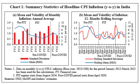
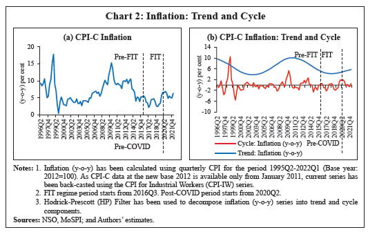 In the post-COVID period, due to unanticipated fluctuations in both supply and demand, mean inflation increased significantly while inflation volatility subsided. As a result, trend inflation8 started rising, reversing its course of a sustained fall since 2011 (Chart 2). Like many other economic crises, the pandemic might also have introduced structural changes in the inflation process. A formal structural break test on headline inflation indeed suggests a break which coincided with the onset of the pandemic (Chart 3 (a)). Reflecting these changes, the dynamic correlations of headline inflation with its own lags have also changed, suggesting the existence of some non-linearities (Chart 3 (b)). In order to better capture these observed changing properties of the inflation data and generating reliable short-term forecasts, this paper attempts to explore ML techniques which are considered more suitable in capturing such non-linearities. Accordingly, this paper employs both traditional time series models and ML techniques to examine their forecasting performance over one-quarter ahead and four-quarters ahead. Section III
Literature Review Alternative forecasting techniques have their own advantages and disadvantages. Linear econometric models are interpretable in the sense that the impact of each explanatory variable on the target variable can be observed, although the degree of interpretability varies across different techniques. However, many studies (Barkan et al., 2022; Sanyal and Roy, 2014 and Nakamura, 2005) suggest that linear models may fail to capture possible non-linearities, business cycles and volatility in the data properly. Machine Learning offers a set of techniques that can usefully summarise various non-linear relationships in the data (Varian, 2014). They also allow us to explore different optimisation methods other than Ordinary Least Squares (OLS)9. More recently, many studies have proposed ML algorithms as an alternative to statistical models for forecasting (Pratap and Sengupta, 2019); these algorithms have become a popular forecasting tool due to the growing availability of big databases and computing power, and greater access to specialised software (Rodríguez-Vargas, 2020). More specifically, universal approximators like neural networks are capable of capturing and dealing with non-linearities (Binner et al., 2005 and Hornik et al., 1989). The use of ML techniques has become popular and widely accepted in recent years. According to a recent survey conducted among the members of the Irving Fischer Committee (IFC), Big Data and Machine Learning applications are discussed formally and widely in most central banks, and are being used in a variety of areas, including research, monetary policy and financial stability (Doerr et al., 2021 and Serena et al., 2021). The use and discussion around these terminologies and methods have increased as per the recent survey of IFC members as compared to a similar survey in 2015 (Tissot et al., 2015). Varian (2014) argues that ML techniques such as neural-nets, decision trees, support vector machines, and so on may allow for more effective ways to model complex relationships. Traditional econometric models may not deliver consistent and reliable forecasts, since they are not well-equipped to capture these complexities and therefore, Deep Learning presents itself as a promising approach, given its success in dealing with Big Data and non-linearities and turns out to be superior in terms of consistency and out-of-sample performance (Theoharidis, 2021). In the central banking circle, according to a study at the Bank of England (Chakraborty and Joseph, 2017) on UK CPI inflation data, ML models (especially universal approximators like neural networks) generally outperform traditional modelling approaches in prediction tasks, while research questions remain open regarding their causal inference properties. A similar study by Rodríguez-Vargas (2020) compares several ML techniques with that of an average of univariate inflation forecasts currently used by the Central Bank of Costa Rica to forecast inflation and finds that best performing forecasts are those of RNN-LSTM, univariate KNN (k-nearest neighbours) and, to a lesser extent, random forests. Using the inflation data for the US, Nakamura (2005) finds that neural networks outperform univariate autoregressive models on average for short horizons of one and two quarters. Another study at the European Central Bank (ECB) (McNelis and McAdam, 2004) finds that neural network-based ‘thick’ models10 for forecasting inflation based on Phillips curve formulations outperform the best performing linear models for ‘real-time’ and ‘bootstrap’ forecasts for service indices for the euro area, and performs well or sometimes better, for the more general consumer and producer price indices across a variety of countries. Based on a large dataset from the US CPI-Urban index, evaluations of Barkan et al. (2022) indicate that the Hierarchical Recurrent Neural Network (HRNN)11 model performs significantly better than several well-known inflation prediction baselines. Paranhos (2021) finds that DL techniques like neural nets including RNN-LSTM usually provide better forecasting performance than standard benchmarks, especially at long horizons, suggesting an advantage of the recurrent model in capturing the long-term trend of inflation. On monthly US CPI inflation data, Almosova and Andresen (2019) find that RNN-LSTM-based neural-net model outperforms several traditional linear benchmarks and even the simple fully-connected neural network (NN). In the Indian context, the literature around the use of non-linear ML techniques for the objective of inflation forecasting is rather scarce. Pratap and Sengupta (2019) find that ML techniques generally perform better than standard statistical models in case of inflation forecasting in India. More specifically, neural network models are very successful in predicting non-linear relationships and outperform traditional econometric models (Rani et al., 2017). Using inflation data for India, South Africa and China, Mahajan and Srinivasan (2020) suggest that deep neural networks outperform benchmark models (moving average and SARIMA) and help in reducing inflation forecast error. According to Kar et al. (2021), ML techniques are superior than non-ML alternatives for longer forecast horizons. Since inflation expectations play a role in influencing the actual path of inflation in an economy, inflation generally turns out to be persistent in nature to some extent, which is beneficial for the forecasting exercise. The role of inflation expectations has increased in driving inflation persistence during the post-Global Financial Crisis period (Patra et al., 2014). Therefore, traditional autoregressive models like ARIMA and SARIMA generally perform better than other traditional alternatives. Using Indian inflation data, Jose et al. (2021) find that seasonal ARIMA (SARIMA) models perform better than other traditional alternatives for one-quarter ahead out-of-sample forecast. For the post-COVID period, studies comparing performance of alternative forecasting models for inflation in India are rare. The characteristics of inflation and its relationship with other variables might have changed during this period. Phillips curve-based relations might also have become weaker over time, especially in the post-COVID period with significant changes in the output gap12. This gives us a motivation to undertake a post-COVID period study to compare the performance of alternative forecasting models including ML techniques to check if performance of widely accepted traditional models have changed or ML techniques add any value in the forecasting exercise and reduce forecast errors on Indian inflation data. Section IV
Methodology, Data and Empirical Strategy Headline inflation (y-o-y) in India has undergone changes in terms of its mean and volatility over the medium run, making it non-stationary in nature. However, CPI quarterly momentum13 (q-o-q per cent change in CPI-C) is stationary, and therefore, has been used as the final target variable for empirical exercises in this study (Table 2). All empirical work in the paper is based on quarterly data. For generating out-of-sample forecasts, rolling sample forecast strategy has been used in the paper to control for sample period bias. For this, data till 2018Q4 have been used for selection of model specification for each technique. Thereafter, the finally selected models are run or trained on a rolling basis adding one successive quarter at a time to generate 12 out-of-sample forecasts that are one-quarter ahead (2019Q1-2021Q4) and 10 forecasts that are four-quarters ahead (2019Q4-2022Q1). To generate four-quarters ahead forecasts for each sample period, recursive forecasting method has been used. | Table 2: Brief Overview of the Study Sample | | Item | Traditional Techniques | ML Techniques | | Study Period | 1996Q2-2022Q1 | 1996Q2-2022Q1 | | Model Identification Period | 1996Q2-2018Q4 | 1996Q2-2018Q4 | | Target Variable | CPI momentum (q-o-q) | CPI momentum (q-o-q) | | Frequency | Quarterly | Quarterly | | Test Data Size | - | 8 | | Model Building Period | Training Period | Training + Testing Period | | First Sample Training Data Period | 1996Q2-2018Q4 | 1996Q2-2016Q4 | | First Sample Testing Data Period | - | 2017Q1-2018Q4 | | Notes: CPI momentum (q-o-q) is the q-o-q per cent change in CPI. q-o-q: quarter-on-quarter - implies current quarter over previous quarter. | Machine Learning models generally require a testing data14 to test for the accuracy of models trained on training data and choose optimal one, which has minimum error15 on test data. Choice of test data size depends on multiple factors, including: (i) if model is generalising well on large test data, then it is more reliable; (ii) for near-term forecasts, however, test data size should not be very large but it should contain all the seasons for full representation of the seasonal pattern; and (iii) test data error is sensitive to both test data and its size. Therefore, this paper has used eight quarters for every sample period as testing data. For a like-for-like comparison of ML models with the traditional models, purely out-of-sample forecasts have been generated by including the test data itself in the model building period for every sample period. | Table 3: Brief Description of Techniques | | Technique type | Technique | Non-Linear | | Univariate | Traditional | Random Walk
ARIMA and SARIMA
Linear Regression | No | | ML | Artificial Neural Network (ANN)
Recurrent Neural Network – LSTM | Yes | | Multivariate | Traditional | ARIMAX and SARIMAX
Phillips Curve (Hybrid NKPC)
Vector Autoregression (VAR)
Linear Regression | No | | ML | Artificial Neural Network
Recurrent Neural Network - LSTM | Yes | In this paper, several traditional and ML techniques have been used to create a comprehensive comparison of their forecast performances. Different combinations of forecasts of models with similar performance have also been considered for the comparison. The set of all the techniques can be divided into two broad categories i.e., Univariate and Multivariate which can be further divided into two sub-categories i.e., Traditional and ML-based (Table 3). IV.1 A Brief Overview of Traditional Techniques Random Walk Random walk refers to any process which contains no observable pattern or trend (Patra et al., 2021) and can be defined as a process in which current value of a variable is a sum of its previous value and a white noise error term i.e., yt = yt-1 + et where, yt is value of the target variable at time t and et is error at time t. In case of forecasting, expected errors are assumed to be zero and forecast is simply the repetition of the previous value. Random walk process is generally considered as a benchmark in forecast comparison exercise of alternative models. Linear Regression This technique tries to estimate a linear relationship between target variable and explanatory variables (regressors) using past data which can be further used to forecast path of the target variable. Linear regression can be built between the target variable and its own lags as well to create an autoregressive16 univariate model. A multivariate model can also be built by introducing variables other than the target variable. The general form of model can be expressed as: Autoregressive Time Series Models Autoregressive integrated moving average (ARIMA) considers autoregressive terms (past lags of target variable) and moving average terms (past lags of errors) as explanatory variables to explain variation in target variable and forecast its path. ARIMA-based forecasting has become one of the popular forecasting methods due to its simplicity as it requires only single time-series (Jose et al., 2021). If the target variable is very seasonal in nature, seasonal components should also be considered for better explanation and forecast performance. Seasonal-ARIMA (SARIMA) helps in achieving this objective by introducing seasonal lags of both autoregressive and moving average terms. (S)ARIMAX is an extended form of (S)ARIMA technique which also considers explanatory variables other than the target variable to make it multivariate in nature. The X added in the end stands for “exogenous”. When exogenous explanatory variables are highly significant, they are generally expected to improve the explanatory power of autoregressive models as they may have potential of explaining variation in the target variable better than just the target variable itself. This model structure can be viewed as a combination of (S)ARIMA and linear regression. Phillips Curve Phillips Curve (PC) is an equation that relates the unemployment rate, or some other measure of aggregate economic activity, to a measure of the inflation rate (Atkeson and Ohanian, 2001). The Phillips curve says that unemployment can be lowered (output can be increased) but only at the cost of higher wages (inflation) and vice versa (Patra et al., 2021). The backward-looking PC has been relied upon by many macroeconomic forecasting models and continues to be the best way to understand policy discussions about the rates of unemployment and inflation, regardless of ample evidence that its forecasts do not improve significantly upon good univariate benchmarks (Stock and Watson, 2008). The literature on PC has evolved significantly overtime, with the New-Keynesian Phillips Curve (NKPC) and its appealing theoretical micro-foundations gaining attention (Nason and Smith, 2008 and Dees et al., 2009). In case of India, the literature supports the existence of PC relationship and an empirical examination of the slope of the PC suggests that the relationship remains relevant as the time-varying output gap coefficient is found to be reasonably stable (Pattanaik et al., 2020). As the inflation process in India has become increasingly sensitive to forward-looking expectations (Patra et al., 2021), the hybrid NKPC has gained popularity as the more appealing specification since it considers the inflation expectations as both forward and backward looking (Gali and Gertler, 1999 and Gali et al., 2005). Therefore, hybrid NKPC has been used in the paper for the performance comparison. Drawing from Indian literature, trend inflation has been used as a proxy for inflation expectation (Jose et al., 2021 and Patra et al., 2021). Vector Autoregression (VAR) Vector Autoregression (VAR) is a set of dynamic statistical equations involving a set of variables where every variable is used to determine every other variable in the model (Pesaran and Henry, 1993). It is a modelling and forecasting technique which is used when simultaneity is present among the target and other variables, i.e., when the target variable and explanatory variable tend to cause or impact each other. VAR technique tries to estimate simultaneity-adjusted coefficients of the variables and is flexible enough to consider exogenous variables as well in the model. Modelling multiple time-series variables simultaneously along with inflation using VARs is a popular approach (Bańbura et al., 2010 and Canova, 2011). IV.2 Overview of ML Techniques In this paper, only DL has been used to represent the ML techniques. It is a subset of Machine Learning which further is one of the branches of Artificial Intelligence (Chart 4). Under Machine Learning (ML), two types of learning techniques are present i.e., supervised learning and unsupervised learning (Chart 5). Supervised learning is an approach where a computer algorithm or technique is trained on data which is properly labelled in the sense that distinction between input and output variables can be made. Under this, as among others, DL, random forest, decision trees, and Support Vector Machines (SVM) are mainly considered. On the other hand, unsupervised learning is suitable when data is raw and not labelled. Clustering is a popular technique under unsupervised learning which focuses on creating groups or clusters using any suitable metric according to study requirements. Since this paper works on economic data which are properly labelled, only supervised learning techniques have been considered. 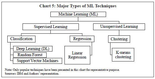 Under DL, although several popular techniques are present, like artificial neural networks (ANN), convolutional neural networks (CNN)17, and recurrent neural networks (RNN), only ANNs and RNNs have been considered in this paper due to simplicity of ANNs, sequential nature of RNNs and data suitability. Within RNNs, only RNN-LSTM has been considered due to its ability to capture longer memory18. Artificial Neural Network (ANN) Artificial neural networks (ANNs) are deep learning algorithms (a subset of ML) whose name and structure are inspired by the human brain as they try to mimic the way biological neurons signal to one another. The structure of ANNs consists of node19 layers, containing an input layer, one or multiple hidden layers, and an output layer (Chart 6). Each node (unit or artificial neuron) is connected to others and has an attached weight and if the output of any individual node is above the specified threshold value, that neuron is activated, sending data to the next layer of the network (IBM Cloud Education, 2020). The idea of neural network comes from McCulloch and Pitts (1943) who modelled the biological working of an organic neuron in a first ever artificial neuron to show how simple units could replicate logical functions. After years of evolution, neural nets became popular with the work of Rumelhart et al. (1986). Last decade has seen a significant rise of DL. ANN architecture can be understood as an advanced and generalised case of logistic regression model whose architecture can be viewed as a specific case of an ANN having single hidden layer with single node. Architecture of ANN has been designed to capture possible non-linearities and dynamic relationships present in the data. DL models contain several hyper-parameters20. To understand the ANN process, one can look at a specific representation having one hidden layer with two nodes/units without constant terms (bias) (Chart 6). A constant term (bias) can also be added at every layer. It may be noted that several hidden layers with several neurons can be used depending on the requirements of user, data availability and the study complexity. Multiple layers with several nodes are helpful in case of huge datasets.
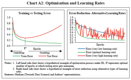
ANN learning process (for the above architecture) can be expressed as follows: A total of eight parameters are present in the model structure (six connecting input to first hidden layer and two connecting hidden layer to the output layer). The objective is to minimise the error with respect to all the eight parameters. Since the error function is non-linear and complex, multiple local minima could be present and therefore, the OLS method cannot be used here. A method called gradient descent is generally used in such cases in the learning process which can be understood as f ollows: 1. Random initial values of parameters are introduced in the first iteration. Using them, error is calculated and accordingly parameters are revised with the following rule: New value of parameter = Old value of parameter – Learning Rate23 * Gradient 2. This process is revised repeatedly until the values of parameters converge to an optimal set of values such that the error gets minimised. One round of revision of parameters is one epoch. This whole learning process is an example of what is called gradient descent with back-propagation i.e., computation of gradients with respect to all parameters and iteratively moving towards global minimum of error function using learning rate and computed gradients by going back from output layer to input layer repeatedly. Recurrent Neural Network (RNN) The primary difference between ANN and RNN is that the latter involves learning both cross-sectionally and inter-temporally (across observations). Architecture of RNN is similar to that of ANN except that it attaches a parameter on previous observations also. RNNs do this by accepting input not only from the current input in a sequence but also from the state of the network that arose when considering previous inputs in that sequence (Hall and Cook, 2017). To understand RNN process, a simple and specific example of a RNN with one input variable and one hidden layer with single node has been considered. Due to its sequential nature, architecture of a RNN is better understood in its unrolled form (Chart 7). At every time point t, a linear combination of previous state ht-1 and current value of input variable xt is taken using parameters U and W. The output is then compared with corresponding actual value of output variable (yt) to calculate error. This process is repeated to minimise error over time and find optimal values of U, V and W. This whole learning process uses what is generally called as back-propagation through time. RNNs face a problem called vanishing/exploding gradients in the learning process which has been explained as follows: The objective is to minimise a loss function (L), which can be defined as sum of squared errors or in any suitable form, with respect to all the parameters. Using back-propagation, gradients with respect to all parameters U, V and W are computed. However, calculating the gradient with respect to U (parameter associated with time state) can be challenging as illustrated below: In (3), parameter U gets multiplied with itself several times. This implies that when U < 1, gradients vanish and if U > 1, gradients explode. Both of these scenarios affect the learning process; this problem is known as short-term memory problem of RNNs. RNN-Long Short-Term Memory (RNN-LSTM) attempts to solve this problem which can learn from long sequences, while the vanilla RNN may not (Mahajan and Srinivasan, 2020). Recurrent Neural Network – Long Short-Term Memory (RNN-LSTM) RNN-LSTM has the capacity to store and capture a longer memory of a sequence along with short-run memory of the most recent network outputs (Hall and Cook, 2017). They are simply recurrent neural networks with some adjustment such that they do not suffer from a short-term memory problem. This model structure was first introduced by Hochreiter and Schmidhuber (1997) and the intuition behind this algorithm relies on the existence of a hidden cell state that tends to be more stable when compared to its counterpart in the plain RNN, leading to more stable gradients and this stability arises from the additive nature of the cell state, as well as the presence of filters or gates that attempt to control the flow of information (Paranhos, 2021). This implies that even if some gradients get close to zero or explode during repeated multiplication while solving minimisation problem, additive term value can be scaled up or down such that gradients do not vanish or become too small or explode. The feature of ‘long memory’ and its ability in using information far in the past makes the LSTM model attractive and differentiates it from the plain RNN model (Paranhos, 2021). IV.3 Data and Variable Selection The paper uses the CPI-C data at the base year 2012 published by the National Statistical Office (NSO), MoSPI, Government of India. As data at the new base 2012 is available only from January 2011, current series has been back-casted till 1995Q2 using the CPI for Industrial Workers (CPI-IW) series. CPI momentum (q-o-q per cent change in CPI) has been used as the target variable for two reasons. First, CPI-C inflation rate (y-o-y) in India has undergone changes in its mean and volatility over the medium run, making it non-stationary in nature. The Augmented Dickey Fuller (ADF) test has been used to check stationarity (Table 4). Second, year-on-year numbers are often impacted significantly by base effects (i.e., change observed during the same period of last year). Therefore, index values have been converted to quarterly momentums (q-o-q per cent change in CPI). No seasonal adjustment has been done in the data due to three reasons. First, the paper has concentrated only on forecasting and not impact assessment. Second, seasonality helps in forecasting. Any seasonal variation can be explained by using the same season lag and alternate seasonal lags. Third, seasonally adjusted data miss out information on seasonality and forecasts created using seasonally adjusted data require re-seasonalisation or forecast of seasonality. Seasonal adjustment process always results in loss of some information, even when it is conducted properly (IMF, 2017). However, seasonally adjusted data has been used in case of linear multivariate macroeconomic models like PC based models to identify economic relationships and VAR model also. Seasonal adjustment has been done using Census X-13 method24. Seasonal average25 has also been used as an explanatory variable for some models to control for static seasonality. | Table 4: Stationarity Tests | | Variable | ADF Test Statistic | P-value | Result | | Inflation (y-o-y) | -1.93 | 0.61 | Non-stationary | | CPI momentum (q-o-q) | -3.24* | 0.08 | Stationary | Notes: 1. Data on inflation (y-o-y) and CPI momentum (q-o-q) has been calculated using CPI-C (1995Q2-2022Q1) with the latest base (2012).
2. *: P < 0.10; **: P < 0.05; ***: P < 0.01
Source: Authors’ estimates. | Following the empirical literature in case of India (Dua and Goel, 2021 and Mohanty and John, 2015), for the multivariate modeling exercise, information on exchange rate, money supply, crude oil price, output gap, rainfall deviation, global food and non-fuel prices, minimum support prices (MSPs), global supply chain pressure index, agricultural wage and call money rates (WACR) has been considered. Explanatory variables and their appropriate lags for each model have been selected keeping multiple factors in mind i.e., theoretical significance, statistical significance and correlations. For identification of variables with statistical significance, the forward selection26 technique has been used. Statistical significance check is important for multivariate linear models to narrow down the count of explanatory variables. In case of algorithms like neural nets, large number of variables can be included as they are capable of using different combinations of variables via multiple nodes/units. A total of 11 explanatory variables (other than inflation) have been considered for the empirical exercise (Table 5). IV.4 Model Selection In traditional techniques, the choice of autoregressive time series (ARIMA and SARIMA) and regression models is based on Akaike Information Criterion (AIC). In case of ARIMAX and SARIMAX, only the most important exogenous variables (identified in variable selection exercise) have been additionally introduced till the model AIC reached its minimum. For PC and VAR, the paper follows the choice of variables as made in Jose et al. (2021). | Table 5: Description of Explanatory Variables | | | Explanatory Variables | Source | | Domestic | Money Supply momentum (M3) | Reserve Bank of India (RBI) | | Output (GDP) Gap (%) | MoSPI, GoI, Authors’ estimates | | Rainfall Deviation from LPA (%) | IMD, GoI | | Minimum Support Price (MSP) momentum | CACP, GoI | | Agricultural Wage Rate momentum | Labour Bureau, MLE, GoI | | Weighted Average Call Money Rate (FD) | Reserve Bank of India (RBI) | | Global | Exchange Rate momentum | FBIL | | Crude Oil Price momentum | MoPNG, GoI | | Global Food Price Index momentum | International Monetary Fund | | Global Non-Fuel Price Index momentum | International Monetary Fund | | Global Supply Chain Pressure Index momentum | Federal Reserve, US | Notes: 1. IMD: Indian Meteorological Department; CACP: Commission on Agricultural Costs and Prices; MLE: Ministry of Labour and Employment; FBIL: Financial Benchmarks India Pvt. Ltd.; MoPNG: Ministry of Petroleum and Natural Gas. LPA: Long Period Average; FD: First Difference.
2. In the table, momentum implies quarter-over-quarter per cent change.
3. MoSPI does not provide data on output gap.27 To calculate the output gap, the Hodrick-Prescott (HP) Filter has been used to decompose GDP series into trend and cyclical components. | In DL models28, after selection of final input variables, the choice of hyper-parameters plays an important role in the training process. Using different range of values of different hyper-parameters, several specifications have been created using same set of input variables. For final choice of hyper-parameters, each specification has been trained on first sample training data (1996Q2 – 2016Q4) and its in-sample forecast accuracy has been evaluated on first sample testing data (2017Q1 – 2018Q4). Root mean squared error (RMSE) has been used to evaluate the forecast accuracy. To control for the impact of random initial values of parameters (weights), each specification was run for 500 times and then average RMSE was calculated. The specification with lowest average RMSE has been chosen for the out-of-sample forecasting exercise. After selecting the final model specification for each technique (Annex Table A1 and A2), each model has been run or trained on rolling sample basis adding one successive quarter at a time until the end of the sample period. Section V
Results The paper has compared several techniques with different characteristics i.e., univariate traditional, univariate ML-based, multivariate traditional and multivariate ML-based techniques. ML techniques have been represented by the DL techniques. As the out-of-sample forecasts are in the quarter-on-quarter (q-o-q) momentum form, they have been converted into year-on-year (y-o-y) numbers for like-to-like comparison with respect to actual inflation rates (y-o-y) and median forecasts (y-o-y) of survey of professional forecasters (SPF). In case of every model, root mean squared error (RMSE) of out-of-sample forecasts has been calculated for pre-COVID, post-COVID and the full period. Average RMSEs of individual models for each model type have also been calculated for performance comparison among model types. V.1 Performance Comparison with Respect to Actual Inflation Forecast Comparison: Individual Models and their Combinations In case of one-quarter ahead comparison, univariate ANN outperforms other models in all periods (Table 6). For full sample forecast period, univariate ANN outperforms the others followed by univariate linear regression and multivariate ANN. In the pre-COVID period, both univariate ANN and univariate linear regression outperform all other models, followed by the ARIMA model. In post-COVID period, after univariate ANN, multivariate ANN and then univariate linear regression outperform the remaining ones. Within traditional techniques, univariate linear regression is the best performer for the full period followed by SARIMA, ARIMA and multiple linear regression. This performance of linear regression can be attributed to the inclusion of only the significant lags identified using forward selection technique rather than including lags in sequence as the autoregressive part, as is done under the ARIMA, SARIMA and VAR models. When all the sequential lags are included, the technique is forced to attach parameters to in-between insignificant lags as well which affects the forecast as compared to the case where only significant lags are included. | Table 6: Performance Comparison of Alternative Models vis-à-vis Actual Inflation | | RMSE of Rolling Sample Forecasts of Inflation (y-o-y) vis-à-vis Actual Inflation | | Model Type | Model | One-quarter ahead
(2019Q1-2021Q4) | Four-quarters ahead
(2019Q4-2022Q1) | | Full period | Pre-COVID | Post-COVID | Full period | Pre-COVID | Post-COVID | | Univariate | Traditional | Random Walk | 0.92 | 1.07 | 0.76 | 2.53 | 3.04 | 1.44 | | ARIMA | 0.80 | 0.71 | 0.87 | 1.25 | 1.43 | 0.91 | | SARIMA | 0.79 | 0.74 | 0.84 | 1.57 | 1.89 | 0.91 | | LR | 0.66 | 0.61 | 0.70 | 0.93 | 0.87 | 1.00 | | ML | ANN | 0.58 | 0.61 | 0.55 | 0.93 | 0.97 | 0.87 | | RNN-LSTM | 0.76 | 0.72 | 0.80 | 1.77 | 1.90 | 1.55 | | Multivariate | Traditional | ARIMAX | 0.82 | 0.79 | 0.86 | 1.60 | 1.81 | 1.21 | | SARIMAX | 0.97 | 0.85 | 1.08 | 1.39 | 1.62 | 0.96 | | PC (Hybrid NKPC) | 1.53 | 0.99 | 1.93 | 2.23 | 1.74 | 2.81 | | VAR | 1.13 | 1.10 | 1.16 | 1.00 | 0.79 | 1.25 | | VAR (SA data) | 1.76 | 1.28 | 2.13 | 1.94 | 1.66 | 2.30 | | LR | 0.80 | 0.84 | 0.76 | 1.01 | 0.84 | 1.21 | | ML | ANN | 0.71 | 0.77 | 0.65 | 1.26 | 1.49 | 0.80 | | RNN-LSTM | 0.93 | 0.89 | 0.97 | 1.60 | 1.84 | 1.16 | | | | Combinations | ANN (U) + LR (U) | 0.59 | 0.60* | 0.59 | 0.88* | 0.87 | 0.90 | | ANN (U) + ANN (M) | 0.61 | 0.65 | 0.56 | 0.94 | 1.19 | 0.32* | | ANN (U) + LR (M) | 0.63 | 0.67 | 0.59 | 0.63* | 0.71* | 0.47* | | LR (U) + ANN (M) | 0.64* | 0.65 | 0.63* | 0.88* | 1.09 | 0.37* | | LR (U) + LR (M) | 0.69 | 0.71 | 0.67 | 0.74* | 0.79* | 0.65* | | LR (M) + ANN (M) | 0.72 | 0.77 | 0.67 | 0.97* | 0.98 | 0.96 | Notes: 1. LR: Linear Regression; PC: Phillips Curve; SA: Seasonally Adjusted. U: Univariate; M: Multivariate.
2. For one-quarter ahead forecast, Full period length is 12 quarters, Pre-COVID period length is 6 quarters, Post-COVID period length is 6 quarters.
3. For four-quarters ahead forecast, Full period length is 10 quarters, Pre-COVID period length is 6 quarters, Post-COVID period length is 4 quarters.
4. Combinations have been calculated using simple average of forecasts of individual models. * indicates improvement with forecast combination if RMSE (Combination) < Minimum (RMSEs of individual models).
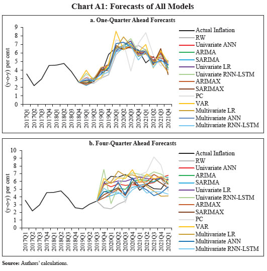
Source: Authors’ estimates. | Within ML techniques, ANNs outperform RNN-LSTMs, which could be due to two reasons: First is the difference in the design of RNN-LSTM that assigns a constant (same) weight to previous hidden states. Even with seasonal volatility (particularly, differential transitions between seasons) present in the target variable (q-o-q per cent change in the CPI), it uses the same weight to calculate the out-of-sample values and ends up producing a sub-optimal forecast. In case of inflation (y-o-y) or non-seasonal variables as target variables where fluctuations are less, LSTM may add value. In other words, LSTM tries to optimise both cross-sectionally and sequentially (across observations), while ANNs (non-sequential) only optimise cross-sectionally. Here, the application of sequential optimisation on the used data has probably led to the suboptimal performance of LSTM. Second, the small data size could also be a limiting factor in case of LSTMs, as they contain larger number of parameters than ANNs and can result in over-parameterisation. Despite these differences, both techniques have been used in the paper to cover newer developments like sequential algorithms within the DL category for drawing robust conclusions. For a comparison of the forecasts that are four-quarters ahead, both univariate ANN and univariate linear regression are the best performers for the full sample period followed by the VAR model. In the pre-COVID period, the VAR model outperforms others, followed by multiple linear regression and univariate linear regression. In the post-COVID period, multivariate ANN outperforms others, followed by univariate ANN and ARIMA/SARIMA models. When the combination forecasts are compared with the individual forecasts in the one-quarter ahead horizon, the univariate ANN emerges again as the best performer. Although the combination forecasts for the four-quarter ahead horizon yield lower RMSEs, this could be due to the errors on the upside under one model getting cancelled out by the errors on the downside under another model, and therefore it may not be possible to draw any definitive conclusion about their forecasting performance. On the whole, the forecasts of univariate ANN were generally seem to be better aligned with the actuals over the short horizon than the autoregressive time series models. Over a four-quarter ahead horizon too, ANN picked up the turning point in 2019Q4, which enabled it to yield lower errors over the further periods than other models. Moreover, during this period, ANN forecasts were directionally more consistent than the others with the actual headline inflation (Chart 8). The forecast comparison for all the models is presented in the Annex (Chart A1). Forecast Comparison: Model Types In view of multiple competing models within each category, an analysis is also undertaken to evaluate forecast performance by model-type by taking simple average of RMSEs of individual models belonging to each model type. The results show that the ML techniques outperform the traditional ones over both horizons in the post-COVID period (Table 7). Over the one-quarter ahead horizon, as expected, univariate models perform better than multivariate ones across all periods. In the post-COVID period, over both horizons, multivariate models significantly underperform probably due to the change in the lag structure of explanatory variables reflecting the presence of uncertainty. 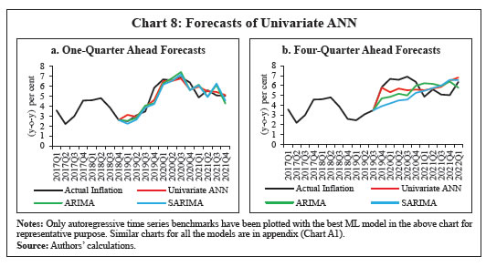
| Table 7: Performance Comparison of Alternative Model Types vis-à-vis Actual Inflation | | Average RMSE of Rolling Sample Forecasts by Model-Type vis-à-vis Actual Inflation | | Model Type | One-Quarter Ahead
(2019Q1-2021Q4) | Four-Quarters Ahead
(2019Q4-2022Q1) | | Full Period | Pre-COVID | Post-COVID | Full Period | Pre-COVID | Post-COVID | | Univariate | 0.75 | 0.74 | 0.75 | 1.50 | 1.68 | 1.11 | | Multivariate | 1.08 | 0.94 | 1.19 | 1.50 | 1.47 | 1.46 | | Traditional | 1.02 | 0.90 | 1.11 | 1.55 | 1.57 | 1.40 | | ML | 0.75 | 0.75 | 0.74 | 1.39 | 1.55 | 1.10 | Notes: 1. For one-quarter ahead forecast, Full period length is 12 quarters, Pre-COVID period length is 6 quarters, Post-COVID period length is 6 quarters.
2. For four-quarters ahead forecast, Full period length is 10 quarters, Pre-COVID period length is 6 quarters, Post-COVID period length is 4 quarters.
Source: Authors’ estimates. | V.2 A Comparison with the Forecasts from Survey of Professional Forecasters (SPF) Individual Models and their Combinations ANN forecasts are closer to those of SPF in case of the one-quarter ahead horizon (Table 8). For the full sample period, across all the techniques, the univariate ANN outperforms other models, followed by ARIMAX and multivariate ANN. In the pre-COVID period, univariate ANN again outperforms others, followed by univariate RNN-LSTM, multivariate RNN-LSTM and SARIMA. In the post-COVID period, multivariate ANN is the best performer, followed by univariate ANN and ARIMAX. Within traditional techniques, ARIMAX is the best performer for the full period, followed by SARIMA and univariate linear regression. In the pre-COVID period, SARIMA outperformed others, followed by the ARIMA model and univariate linear regression. In the post-COVID period, ARIMAX outperformed the others. Within ML techniques, ANNs outperformed RNN-LSTMs. No combination has been able to beat the univariate ANN. | Table 8: Performance Comparison of Alternative Models vis-à-vis SPF (Median) | | RMSE of Rolling Sample Forecasts of Inflation (y-o-y) vis-à-vis SPF (Median) | | Model Type | Model | One-Quarter Ahead
(2019Q1-2021Q4) | Four-Quarters Ahead
(2019Q4-2022Q1) | | Full period | Pre-COVID | Post-COVID | Full period | Pre-COVID | Post-COVID | | Univariate | Traditional | Random Walk | 1.30 | 1.56 | 0.97 | 2.19 | 2.09 | 2.33 | | ARIMA | 0.94 | 0.66 | 1.15 | 1.89 | 1.81 | 2.00 | | SARIMA | 0.86 | 0.63 | 1.05 | 1.63 | 1.30 | 2.02 | | LR | 0.89 | 0.67 | 1.06 | 2.31 | 2.39 | 2.19 | | ML | ANN | 0.70 | 0.47 | 0.87 | 1.89 | 1.80 | 2.01 | | RNN-LSTM | 0.95 | 0.62 | 1.19 | 2.78 | 2.85 | 2.68 | | Multivariate | Traditional | ARIMAX | 0.82 | 0.72 | 0.90 | 1.85 | 1.63 | 2.14 | | SARIMAX | 0.91 | 0.69 | 1.08 | 1.55 | 1.45 | 1.69 | | PC (Hybrid NKPC) | 1.31 | 0.93 | 1.61 | 2.98 | 2.43 | 3.66 | | VAR | 1.12 | 1.06 | 1.18 | 2.58 | 2.66 | 2.46 | | VAR (SA data) | 1.50 | 1.17 | 1.76 | 2.89 | 2.77 | 3.06 | | LR | 1.05 | 1.05 | 1.04 | 2.30 | 2.82 | 1.14 | | ML | ANN | 0.83 | 0.81 | 0.86 | 1.47 | 1.76 | 0.85 | | RNN-LSTM | 0.91 | 0.63 | 1.11 | 1.09 | 1.27 | 0.76 | | | | Combinations | ANN (U) + ANN (M) | 0.73 | 0.62 | 0.83* | 1.59 | 1.73* | 1.34 | | LR (U) + ANN (M) | 0.82* | 0.70 | 0.93 | 1.81 | 2.03 | 1.44 | | LR (U) + LR (M) | 0.93 | 0.86 | 1.01* | 2.22* | 2.59 | 1.49 | Notes: 1. LR: Linear Regression; SA: Seasonally Adjusted; U: Univariate; M: Multivariate; SPF: Survey of Professional Forecasters.
2. For one-quarter ahead forecast, Full period length is 12 quarters, Pre-COVID period length is 6 quarters, Post-COVID period length is 6 quarters.
3. For four-quarter ahead forecast, Full period length is 10 quarters, Pre-COVID period length is 6 quarters, Post-COVID period length is 4 quarters.
4. Combinations have been calculated using simple average of forecasts of individual models. * indicates improvement with forecast combination if RMSE (Combination) < Minimum (RMSEs of individual models).
Source: Authors’ estimates. |
| Table 9: Performance Comparison of Alternative Model Types vis-à-vis SPF (Median) | | Average RMSE of Rolling Sample Forecasts by Model-Type vis-à-vis SPF (Median) | | Model Type | One-Quarter Ahead
(2019Q1-2021Q4) | Four-Quarters Ahead
(2019Q4-2022Q1) | | Full Period | Pre-COVID | Post-COVID | Full Period | Pre-COVID | Post-COVID | | Univariate | 0.94 | 0.77 | 1.05 | 2.12 | 2.04 | 2.21 | | Multivariate | 1.06 | 0.88 | 1.19 | 2.09 | 2.10 | 1.97 | | Traditional | 1.07 | 0.91 | 1.18 | 2.22 | 2.14 | 2.27 | | ML | 0.85 | 0.63 | 1.01 | 1.81 | 1.92 | 1.58 | Notes: 1. For one-quarter ahead forecast, Full period length is 12 quarters, Pre-COVID period length is 6 quarters, Post-COVID period length is 6 quarters.
2. For four-quarters ahead forecast, Full period length is 10 quarters, Pre-COVID period length is 6 quarters, Post-COVID period length is 4 quarters.
Source: Authors’ estimates. | For four-quarters ahead, the forecasts of multivariate RNN-LSTM turn out to be closest to those of SPF in all periods. Among the traditional techniques, SARIMAX outperforms others, followed by SARIMA and ARIMAX for the full period. In the pre-COVID period, SARIMA outperforms others, followed by SARIMAX and ARIMAX. In the post-COVID period, multivariate linear regression is the best performer, followed by SARIMAX and ARIMA. No combination has been able to beat the multivariate RNN-LSTM. Forecast Comparison: Model Types An evaluation by model type suggests that forecasts from ML techniques are closer to SPF forecasts than those based on the traditional techniques for both one-quarter ahead and four-quarters ahead horizons (Table 9). Between univariate and multivariate models, univariate models perform better for the one-quarter ahead forecast horizon. Section VI
Conclusions This paper explored the application of the ML techniques for inflation forecasting and compared their forecasting performance, measured by estimated RMSEs, with the popular traditional models. The empirical results suggest performance gains in using DL (a supervised ML technique) models over the traditional models for different forecast horizons. On an average, ML techniques outperformed the traditional linear models for both the pre-pandemic and post-pandemic periods. The performance gains achieved using the ML techniques over the one-quarter ahead and four-quarters ahead forecast horizons were significantly higher in the post-pandemic period, implying that ML techniques may be better in capturing the pandemic time volatility in inflation. Using the SPF as the target (instead of actual inflation), a similar conclusion emerges, i.e., forecasts of DL models are closer to SPF median forecasts than those from the traditional models. However, given the standard limitations of the ML models – complex structure, over-parameterisation and lack of easy interpretability – a regular assessment of forecast comparison of ML techniques with the traditional models under different sample periods may be necessary. References Abdullah, T. A. A., Zahid, M. S. M., & Ali, W. (2021). A Review of Interpretable ML in Healthcare: Taxonomy, Applications, Challenges, and Future Directions. Symmetry, Multidisciplinary Digital Publishing Institute (MDPI). Almosova, A., & Andresen, N. (2019). Non-linear inflation forecasting with recurrent neural networks: Technical Report, European Central Bank (ECB). Arrieta, A. B., Rodriguez, N. D., Ser, J. D., Bennetot, A., Tabik, S., Barbado, A., Garcia, S., Lopez, S. G., Molina, D., Benjamins, R., Chatila, R., & Herrera, F. (2020). Explainable Artificial Intelligence (XAI): Concepts, Taxonomies, Opportunities and Challenges toward Responsible AI. Information Fusion., 58 (2020), 82-115. Atkeson, A., & Ohanian, L. (2001). Are Phillips curves useful for forecasting inflation? Quarterly Review of Federal Reserve Bank of Minneapolis, 25, 2-11. Blagrave, P. & Lian, W.(2020). India’s Inflation Process Before and After Flexible Inflation Targeting. IMF Working Papers WP/20/251. Bańbura, M., Giannone, D., & Reichlin, L. (2010). Large Bayesian VARs. Journal of Applied Econometrics, 25(1), 71-92. Barkan, O., Benchimol, J., Caspi, I., Cohen, E., Hammer, A., & Koenigstein, A. (2022). Forecasting CPI Inflation Components with Hierarchical Recurrent Neural Networks. International Journal of Forecasting. Bates, J. M., & Granger, C. W. (1969). The combination of forecasts. Journal of the Operational Research Society, 20(4), 451–468. Behera, H. K., & Patra, M. D. (2020). Measuring Trend Inflation in India. RBI Working Paper Series WPS (DEPR): 15/2020 Bhoi, B. K., & Behera, H. K. (2016). India’s Potential Output Revisited. RBI Working Paper Series WPS (DEPR): 05/2016. Binner, J. M., Bissoondeeal, R. K, Elger, T., Gazely, A. M., & Mullineux, A. W. (2005). A comparison of linear forecasting models and neural networks: an application to Euro inflation and Euro Divisia. Applied Economics, vol. 37(6), 665-680. Bobeica, E., & Hartwig, B. (2021). The COVID-19 Shock and Challenges for Time Series Models. ECB Working Paper Series, No 2558. Canova, F. (2011). Methods for applied macroeconomic research. Princeton university press. Chakraborty, C., & Joseph, A. (2017). Machine Learning at Central Banks. Bank of England Staff Working Paper No. 674. Chen, Q., Constantini, M., & Deschamps, B. (2016). How accurate are professional forecasts in Asia? Evidence from ten countries. International Journal of Forecasting, Vol. 32, Issue 1, 154-167. Collins, C., Forbes, K., & Gagnon, J. (2021). Pandemic Inflation and Nonlinear, Global Phillips Curves. CEPR VOXEU Column. https://cepr.org/voxeu/columns/pandemic-inflation-and-nonlinear-global-phillips-curves. Dees, S., Pesaran, M. H., Smith, L. V., & Smith, R. P. (2009). Identification of new Keynesian Phillips curves from a global perspective. Journal of Money, Credit and Banking, 41(7), 1481-1502. Doerr, S., Gambacorta, L., & Serena, J. M. (2021). Big Data and Machine Learning in Central Banking. BIS Working Papers No. 930, Bank for International Settlements, (BIS). Dua, P., & Goel, D. (2021). Determinants of Inflation in India. The Journal of Developing Areas 55(2). Fourati, H., Maaloul, R., & Fourati, L. C. (2021). A Survey of 5G Network Systems: Challenges and Machine Learning Approaches. International Journal of Machine Learning and Cybernetics 12(1). Fulton, C., & Kirstin, H. (2021). Forecasting US inflation in real time. Finance and Economics Discussion Series 2021-014. Board of Governors of the Federal Reserve System, Washington DC. Gali, J., & Gertler, M. (1999). Inflation dynamics: A structural econometric analysis. Journal of Monetary Economics, 44(2), 195-222. Gali, J., Gertler, M., & Lopez-Salido, D. (2005). Robustness of the estimates of the hybrid New Keynesian Phillips curve. Journal of Monetary Economics, 52(6), 1107–1118. Goulet Coulombe, P., Leroux, M., Stevanovic, D., & Surprenant, S. (2022). How is machine learning useful for macroeconomic forecasting? Journal of Applied Econometrics, 37(5), 920-964. Hall, A. S., & Cook, T. R. (2017). Macroeconomic Indicator Forecasting with Deep Neural Networks. Federal Reserve Bank of Kansas City Working Paper No. 17-11. Hauzenberger, N., Huber, F., & Klieber, K. (2022). Real-time inflation forecasting using non-linear dimension reduction techniques. International Journal of Forecasting. Hochreiter, S., & Schmidhuber, J. (1997). Long short-term memory. Neural computation, 9(8), 1735–1780. Hornik, K., Stinchcombe, M., & White, H. (1989). Multilayer feedforward networks are universal approximators. Neural Networks Vol. 2, Issue 5, 359-366. IBM (2020). Neural Networks. IBM Cloud Education. IMF. (2017). Quarterly National Accounts Manual: Chapter 7 – Seasonal Adjustment. John, J., Singh, S., & Kapur, M. (2020). Inflation Forecast Combinations – The Indian Experience. Reserve Bank of India Working Paper Series WPS (DEPR): 11/2020. Jose, J., Shekhar, H., Kundu, S., & Bhoi, B. B. (2021). Alternative Inflation Forecasting Models for India – What Performs Better in Practice? Reserve Bank of India Occasional Papers Vol. 42, No. 1: 2021, 71-121. Kar, S., Bashir, A., & Jain, M. (2021). New Approaches to Forecasting Growth and Inflation: Big Data and Machine Learning. Institute of Economic Growth Working Papers No. 446. LeCun, Y., Bengio, Y., & Hinton, G. (2015). Deep Learning. Nature, 521(7553), 436-444. Mahajan, K., & Srinivasan, A. (2020). Inflation Forecasting in Emerging Markets: A Machine Learning Approach. CAFRAL research publications, Centre for Advanced Financial Research and Learning (CAFRAL). McNelis, P., & McAdam, P. (2004). Forecasting inflation with thick models and neural networks. European Central Bank Working Paper Series No. 352/April 2004. Mehrotra, A., & Yetman, J. (2014). How Anchored are Inflation Expectations in Asia? Evidence from Surveys of Professional Forecasters. BIS Papers No. 77, Bank for International Settlements, (BIS). Mohanty, D., & John, J. (2015). Determinants of Inflation in India. Journal of Asian Economics, 36, 86-96. Murphy, K. P. (2012). Machine Learning: A Probabilistic Perspective. MIT Press, United Kingdom. Nakamura, E. (2005). Inflation forecasting using a neural network. Economics Letters 86 (2005), 373–378. Nason, J. M., & Smith, G. W. (2008). Identifying the new Keynesian Phillips curve. Journal of Applied Econometrics, 23(5), 525-551. Nesvijevskaia, A., Ouillade, S., Guilmin, P., & Zucker, J. D. (2021). The accuracy versus interpretability trade-off in fraud detection model. Cambridge University Press, Data & Policy (2021), Vol. 3, e12-1-e12-24. Paranhos, L. (2021). Predicting Inflation with Neural Networks. The Warwick Economics Research Paper Series (TWERPS) 1344, University of Warwick, Department of Economics. Patra, M. D., Khundrakpam, J. K., & George, A. T. (2014). Post-Global Crisis Inflation Dynamics in India, What has Changed? India Policy Forum, 2013–140 (10), 117-191. Patra, M. D., Behera, H. L., & John, J. (2021). Is the Phillips Curve in India Dead, Inert and Stirring to Life or Alive and Well? RBI Bulletin November 2021, 63-75. Pattanaik, S., Muduli, S., & Ray, S. (2020). Inflation Expectations of Households: Do They Influence Wage-price Dynamics in India? Macroeconomics and Finance in Emerging Market Economies, 1-20. Pesaran, B. & Henry, S. G. B. (1993). VAR models of inflation. Bank of England Quarterly Bulletin (May 1993). Pratap, B., & Sengupta, S. (2019). Macroeconomic Forecasting in India: Does Machine Learning Hold the Key to Better Forecasts? Reserve Bank of India Working Paper Series WPS (DEPR): 04/ 2019. Rani, S. J., Haragopal, V. V., & Reddy, M. K. (2017). Forecasting inflation rate of India using neural networks. International Journal of Computer Applications, 158(5), 45–48. Reserve Bank of India. (2014). Report of the Expert Committee to Revise and Strengthen the Monetary Policy Framework (Chairman: Urjit R. Patel), Reserve Bank of India. Reserve Bank of India. (2021). Report on Currency and Finance 2020-21. Rodríguez-Vargas, A. (2020). Forecasting Costa Rican inflation with Machine Learning methods. Latin American Journal of Central Banking (2020), 100012. Rumelhart, D. E., Hinton, G. E. & Williams, R. J. (1986). Learning representations by back-propagating errors. Nature 323, 533–536. Sanyal, A., & Roy, I. (2014). Forecasting major macroeconomic variables in India: Performance comparison of linear, non-linear models and forecast combinations. RBI Working Paper Series No. 11/2014. Serena, J. M., Tissot, B., & Gambacorta, L. (2021). Use of big data sources and applications at central banks. IFC survey report No. 13, Irving Fisher Committee on Central Bank Statistics. Šestanović, T., & Arnerić, J. (2021). Can Recurrent Neural Networks Predict Inflation in Euro Zone as Good as Professional Forecasters? Mathematics, MDPI, vol. 9(19), 1-13. Sousa, R., & Yetman, J. (2016). Inflation expectations and monetary policy. BIS Papers No. 89, Bank for International Settlements, (BIS). Stock, J. H., & Watson, M. W. (2010). Modelling inflation after the crisis. NBER Working Paper No. 16488, National Bureau of Economic Research (NBER). Stock, J. H., & Watson, M. W. (2008). Phillips curve inflation forecasts. NBER Working Paper No. 14322, National Bureau of Economic Research (NBER). Svensson, L. E. O. (1999). Inflation Targeting as a Monetary Policy Rule. Journal of Monetary Economics, Vol. 43(3), 607-654. Theoharidis, A. F. (2021). Forecasting Inflation Using Deep Learning: An Application of Convolutional LSTM Networks and Variational Autoencoders. Insper Institute of Education and Research, São Paulo, Brazil. Tissot, B., Hülagü, T., Nymand-Andersen, P., & Suarez, L. C. (2015). Central banks’ use of and interest in “big data”. IFC survey report No. 3, Irving Fisher Committee on Central Bank Statistics. Varian, H. R. (2014). Big Data: New Tricks for Econometrics. Journal of Economic Perspectives Vol. 28, No. 2, Spring 2014, 3–28.
Annex 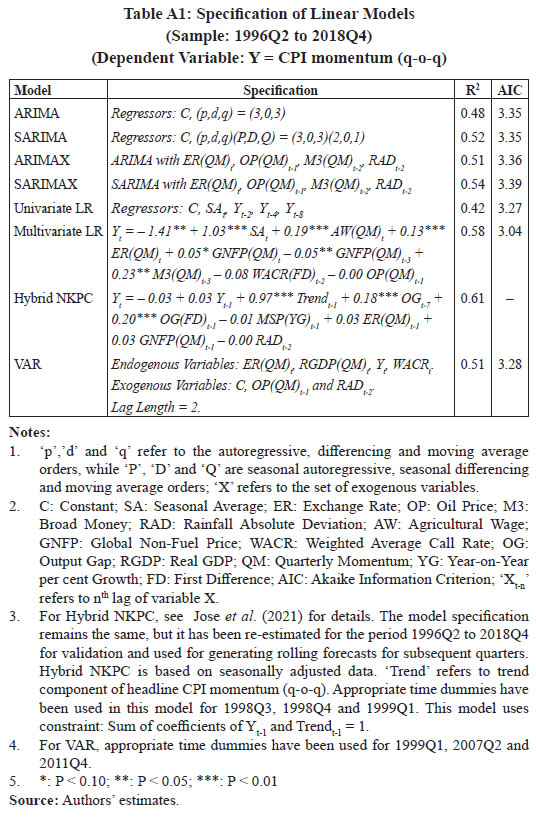
Table A2: Specifications of DL Models
(Sample: 1996Q2 to 2018Q4)
(Dependent Variable: Y = CPI momentum (q-o-q) | | | Univariate ANN | Multivariate ANN | Univariate RNN-LSTM | Multivariate RNN-LSTM | | Structure/ Hyper-parameters | | | | | | Activation function | Sigmoid | Sigmoid | Sigmoid | Sigmoid | | Learning rate | 0.01 | 0.01 | 0.01 | 0.01 | | Number of hidden layers | 1 | 1 | 1 | 1 | | Nodes per hidden layer | 3 | 4 | 2 | 3 | | Maximum epochs | No limit | No limit | 300 | 300 | | Initial weights | Random | Random | Random | Random | | Runs | 500 | 500 | 500 | 500 | | Explanatory Variables | C | C | C | C | | SAt | SAt | SAt | SAt | | Yt-2 | ER(QM)t | Yt-2 | ER(QM)t | | Yt-4 | MSP(QM)t | Yt-4 | MSP(QM)t | | Yt-8 | AW(QM)t-1 | Yt-8 | AW(QM)t-1 | | | OP(QM)t-1 | | OP(QM)t-1 | | | WACR(FD)t-1 | | WACR(FD)t-1 | | | M3(QM)t-2 | | M3(QM)t-2 | | | OGt-2 | | OGt-2 | | | GFP(QM)t-2 | | GFP(QM)t-2 | | | GNFP(QM)t-2 | | GNFP(QM)t-2 | | | RADt-2 | | RADt-2 | Notes:
1. C: Constant; SA: Seasonal Average; ER: Exchange Rate; MSP: Minimum Support Price; AW: Agricultural Wage; OP: Oil Price; OG: Output Gap; GFP: Global Food Price; GNFP: Global Non-Fuel Price; RAD: Rainfall Absolute Deviation; M3: Broad Money; WACR: Weighted Average Call Rate; QM: Quarterly Momentum; FD: First Difference.
2. For simplicity, no decay was applied on learning rate.
3. More number of runs increases probability of finding a better solution as the process reaps benefits from exploring multiple sets of random initial parameters (weights) acting as starting points.
Source: Authors’ estimates. |
|