Indrajit Roy* Received on: August 30, 2022
Accepted on: February 1, 2023 In this paper, a new criterion is proposed to test the presence of a unit root in any zero-mean time series data with no deterministic trend and no structural break. The test is developed based on the ratio of the Probability Density Functions (PDFs) of the data under the null of presence of a unit root to the alternative of stationarity. As the distribution of the test statistic is non-standard, the Monte Carlo simulation (MCS) technique has been used to determine the empirical probability distribution of the test statistic. MCS is also used to compare the power of the test for a finite sample with select univariate unit-root tests that are commonly used in empirical research, namely the ADF test, Phillips-Perron test, KPSS test, ERS test, Zivot and Andrews test, Schmidt and Phillips test, Pantula, Gonzales-Farias and Fuller test, and Breitung’s variance ratio test. The paper demonstrates higher power of the new test vis-à-vis the existing tests for sample sizes under 50. For large sample sizes, its power is either higher or on-par with the other tests. JEL Classification: C22, C53, B23 Keywords: Time series analysis, random walk, Monte Carlo simulation, unit root tests Introduction Any time series data i.e., a sequence of data points arranged to reflect its evolution over time is an integral part of economic analysis, testing of various economic hypotheses, and statistical modelling for forecasting. However, if the time series data are not stationary, then the inferences derived from the analysis can be misleading. If a time series is not stationary, but its first difference is stationary, then the data generating process is called the unit root process. There are many standard methods for testing of unit roots in the literature. The empirical power of these unit root tests, however, is found to be low especially for small samples. The power of a test signifies how well the test can correctly identify a time series as stationary when the series is indeed stationary. This paper proposes a new criterion to test the unit root hypothesis and compares its power with various available unit root tests. The paper is organised as follows: Section II contains a review of the literature, while Section III lays out the methodology for the new test statistic. The test outcome is compared with the other existing tests in Section IV, followed by conclusions in Section V. Section II
Literature Review
There are many tests for the unit root hypothesis testing in autoregressive processes. The commonly used ones are Dickey and Fuller’s ADF test (Dickey and Fuller, 1979); Phillips-Perron test (Phillips and Perron, 1988); KPSS (Kwiatkowski, Phillips, Schmidt and Shin, 1992) test; Elliot, Rothenberg, and Stock (ERS, 1996) test; Zivot and Andrews (ZA, 1992) test; Schmidt and Phillips (SP) test; Pantula, Gonzales-Farias and Fuller (PGFF, 1994) test; and Breitung variance ratio (BVR, 2002) test. To test if a time series is nonstationary, the standard unit-root tests employ model (3) and consider the null hypothesis (H0) and the alternative hypothesis (H1) as follows: H0: β = 1 H1: β < 1 These tests use mainly least-squares estimate (LSE) of β and the test statistic is the t-ratio of the estimate of β and its standard error. The Dickey-Fuller (DF) (Dickey and Fuller, 1979) unit-root test is based on the model of the first-order autoregressive process as in (3). To formulate the test statistic, in equation (3), xt-1 is subtracted from both the sides: Since the right-hand side of equation (5) contains lagged xt i.e., xt-1, the disturbance terms εt are correlated. To take care of the autocorrelation, augmented Dickey-Fuller (ADF) test includes the lagged values of differences of xt in the right-hand side of (5); it also includes a constant term ct, which can be a pure constant or a linear time trend. The Phillips-Perron (PP) unit root test builds on the ADF test but it differs from the ADF test mainly in how it deals with the serial autocorrelation and heteroskedasticity in the errors. The null hypothesis in the PP test assumes that the process has a unit root, and the test statistics are given as follows (Pesaran, 2015): Unlike ADF test, the KPSS test has a null of stationarity of a series including deterministic trend, and the alternative hypothesis is that the series is nonstationary due to the presence of a unit root. According to the KPSS test, time series observations xt are decomposed as the sum of the deterministic trend, a random walk, and a stationary error term. Instead of an LSE of β in equation (1), many studies employ the maximum likelihood estimate (MLE) and observe that the test statistic associated with the exact MLE, under alternative hypothesis of stationarity is more powerful than the LSE used in DF test (Pantula et al., 1994; Fuller, 1996). Skrobotov (2018) investigated the bootstrap implementation of the test as proposed by Jansson and Nielson (2012) and observed that likelihood ratio test produced poor finite sample properties when errors were strongly autocorrelated and noted that as compared to bootstrap ADF, the bootstrap likelihood ratio test exhibited better finite sample properties in certain cases. Section III
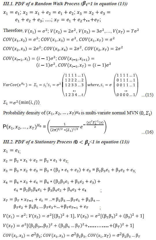
Methodology In this paper, we consider a zero-mean first order autoregressive process i.e., AR (1) with time-varying coefficients as a stationary series as defined in (13), and a nonstationary series (i.e., random walk series) with only stochastic trend component as defined in (14), and develop a test statistic to identify whether a given series is non-stationary (H0) or stationary (H1). AR (1) model is used here with time-varying coefficient (βt) rather than fixed coefficient β to avoid the strong assumptions made by many other studies that xt - β * xt-1 are independent and identically distributed (i.i.d.) with a known distribution, which seems practically implausible. Instead, xt - βt * xt-1 may be more likely i.i.d. in many real applications. The test criterion has been developed assuming the time-varying coefficient (βt) of AR (1) model to make it generic. The test criterion can be applied to a time series irrespective of practitioner’s assumption on time variant coefficients or orders of AR/ MA process. The test criterion is developed assuming that if the observed data series 'x' is indeed generated out of a random walk process, then it would look relatively more probable (or higher likelihood) when fitting it using the PDF of a unit root process rather than force fitting it with the PDF of a stationary process. The critical values or the rejection region of the test statistic is obtained using Monte Carlo Simulation (MCS) method. Further, this paper empirically tests the efficiency of the proposed test in terms of its power, and the proportion of correctly identified series, as compared to other commonly used tests, such as ADF test, Phillips-Perron test, KPSS test, ERS test, Zivot and Andrews (ZA) test, Schmidt and Phillips (SP) test, Pantula, Gonzales-Farias and Fuller (PGFF) test, and Breitung’s variance ratio (BVR) test on a set of simulated stationary (fixed and time-varying AR(1) and AR(2) models) and nonstationary data. Given a time series observation x = (x1, x2, ...,xT), we need to ascertain whether it is generated from a random walk process (null hypothesis: Ho) or a stationary process (Alternative hypothesis: H1). Here, (x1, x2, ..., xT) are not a mere multivariate sample but a time ordered data from a family of random variables. The time series characteristic is embedded in the construction of (x1, x2, ..., xT) and their dependence structure is captured in variance-covariance matrix. The AR (1) stationary series with time-varying parameter as defined in (13) is: 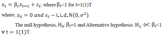

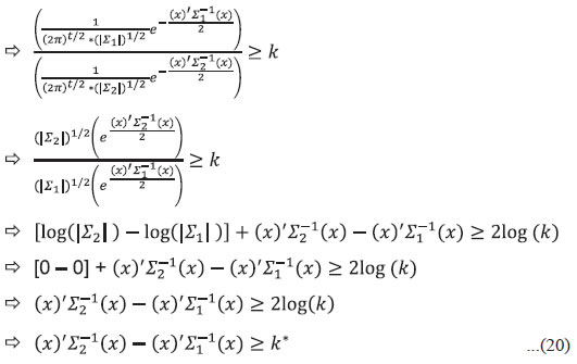 The test statistic (20) proposed in this paper is a linear combination of the non-central chi-squared variables. Its theoretical PDF is complex, and its derivation is beyond the scope of this paper. Therefore, it has been left for future research. Instead of theoretical PDF of the test statistic, the paper uses MCS to derive an empirical probability distribution of the test statistic and the threshold value or critical region is estimated from this empirical PDF. Equation (20) suggests that when the data series x is indeed generated using random walk process, then the observed data x would look more probable (or higher likelihood) while fitting it using the gaussian normal distribution with variance-covariance matrix Σ1 as defined in equation (15) than while trying to force-fit it with a variance-covariance matrix Σ2 as defined in equations (17) or (18). III.4. Estimating the Threshold or Critical Value of the Test Statistic For example, if the sample size is set at 20, and for an instance of a set of βt drawn from the uniform distribution (0,1), the test statistic after arithmetic adjustment becomes: Therefore, the test statistic R20 in (21) can be written as a linear combination of a set of variables which are distributed as chi-squared (X21), and not necessarily independent. The derivation of the exact probability density function of the test statistic is very complex, and is not attempted here. Instead, the MCS-based empirical PDF is used to derive an empirical PDF of the test statistic. We start with a large set (N1) of known non-stationary series of size ‘T’ generated using equation (14) and calculate the test statistic (RT) for each of these N1 non-stationary data series and calculate the empirical probability distribution of the test statistic for various quantiles. While calculating the critical values of the test statistic, a known non-stationary dataset is contrasted with a stationary series using equation (19) with unknown parameters (βt). However, βt cannot be consistently estimated based on the sample observations (x2 = β2 * x1 + e2; x3 = β3 * x2 + e3; ...). Therefore, to calculate critical values, βts are assumed here to be a random sample from a uniform distribution U(0.01,0.99). III.5. Power of the Test Statistic To estimate the empirical power of the new test criterion, we generate N2 stationary series using equation (13) and calculate the power as follows: Since we are estimating empirical power of the test based on a known set of stationary series, we need not be concerned about the specifics of alternative hypothesis. We can use the composite alternative hypothesis (βt < 1 for all t); and determine the probability density of the test statistic under the alternative hypothesis, which may be complicated and is not required in this context. Section IV
Empirical Analysis and Comparisons with a Few Other Unit Root Tests IV.1. Empirical Probability Distribution of the Test Statistic 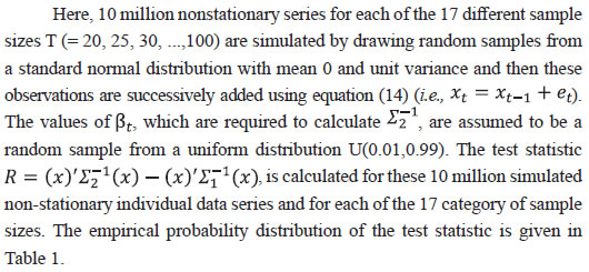
| Table 1: Empirical Probability Distribution of Rt for Non-Stationary Series | | kαT: | Random walk: Empirical pdf of R-test statistic: P[RT αT]H0 = α | | α: 1% | 5% | 10% | 15% | 20% | 25% | 30% | 35% | 40% | 45% | 50% | | T:20 | -4.81 | -0.38 | 3.06 | 6.32 | 9.72 | 13.39 | 17.44 | 21.96 | 27.08 | 32.95 | 39.74 | | 25 | -4.16 | 1.76 | 6.76 | 11.51 | 16.40 | 21.65 | 27.41 | 33.84 | 41.09 | 49.36 | 58.93 | | 30 | -2.64 | 5.75 | 13.25 | 20.43 | 27.86 | 35.86 | 44.65 | 54.47 | 65.54 | 78.17 | 92.75 | | 35 | -0.85 | 10.26 | 20.18 | 29.61 | 39.38 | 49.86 | 61.34 | 74.16 | 88.68 | 105.23 | 124.37 | | 40 | 1.87 | 16.47 | 29.73 | 42.46 | 55.64 | 69.84 | 85.47 | 102.90 | 122.58 | 145.14 | 171.24 | | 45 | 3.59 | 20.08 | 34.96 | 49.20 | 63.95 | 79.86 | 97.37 | 116.86 | 138.99 | 164.30 | 193.59 | | 50 | 6.74 | 26.74 | 44.54 | 61.39 | 78.72 | 97.29 | 117.60 | 140.17 | 165.70 | 194.87 | 228.69 | | 55 | 8.55 | 30.41 | 50.09 | 68.66 | 87.75 | 108.13 | 130.39 | 155.19 | 183.08 | 214.91 | 251.65 | | 60 | 13.33 | 39.64 | 63.28 | 85.65 | 108.55 | 132.99 | 159.63 | 189.18 | 222.40 | 260.14 | 303.62 | | 65 | 19.13 | 51.90 | 81.66 | 109.89 | 138.95 | 169.94 | 203.81 | 241.49 | 283.73 | 331.68 | 386.71 | | 70 | 23.65 | 59.98 | 92.92 | 124.37 | 156.77 | 191.35 | 229.14 | 271.08 | 318.45 | 372.07 | 433.59 | | 75 | 29.51 | 71.11 | 108.87 | 144.77 | 181.76 | 221.33 | 264.65 | 312.71 | 366.74 | 428.31 | 499.08 | | 80 | 34.39 | 80.22 | 121.79 | 161.20 | 201.99 | 245.83 | 293.61 | 346.67 | 406.33 | 474.30 | 552.35 | | 85 | 42.81 | 96.25 | 144.67 | 190.80 | 238.34 | 289.39 | 345.16 | 407.31 | 477.40 | 557.01 | 648.68 | | 90 | 50.51 | 110.45 | 165.06 | 217.11 | 271.05 | 328.76 | 391.93 | 462.30 | 541.56 | 632.05 | 736.10 | | 95 | 56.67 | 121.51 | 180.58 | 236.69 | 294.82 | 357.13 | 425.42 | 501.44 | 587.03 | 684.94 | 797.85 | | 100 | 67.11 | 140.39 | 206.89 | 270.47 | 336.23 | 406.66 | 483.86 | 569.94 | 667.00 | 777.70 | 905.89 |
| kαT: | Random walk: Empirical pdf of R-test statistic: P[RT αT]H0 = α | | 55% | 60% | 65% | 70% | 75% | 80% | 85% | 90% | 95% | 99% | | T:20 | 47.71 | 57.14 | 68.50 | 82.34 | 99.51 | 121.66 | 151.66 | 195.90 | 275.13 | 470.53 | | 25 | 70.14 | 83.37 | 99.24 | 118.57 | 142.68 | 173.71 | 215.55 | 277.43 | 388.53 | 662.01 | | 30 | 109.79 | 129.94 | 154.06 | 183.52 | 220.07 | 267.04 | 330.79 | 424.59 | 593.24 | 1008.64 | | 35 | 146.67 | 173.03 | 204.57 | 243.03 | 290.93 | 352.54 | 435.96 | 559.28 | 779.49 | 1321.08 | | 40 | 201.75 | 237.89 | 281.10 | 333.85 | 399.59 | 484.04 | 598.09 | 766.50 | 1069.18 | 1812.99 | | 45 | 227.84 | 268.31 | 316.91 | 376.17 | 449.99 | 545.08 | 673.45 | 862.20 | 1201.66 | 2035.56 | | 50 | 268.23 | 314.86 | 370.80 | 439.11 | 523.94 | 633.23 | 780.74 | 998.95 | 1390.40 | 2354.68 | | 55 | 294.69 | 345.48 | 406.27 | 480.44 | 572.88 | 691.50 | 852.28 | 1088.75 | 1514.64 | 2563.20 | | 60 | 354.42 | 414.31 | 486.10 | 573.49 | 682.44 | 822.22 | 1010.97 | 1288.91 | 1790.70 | 3023.64 | | 65 | 450.82 | 526.25 | 616.63 | 726.67 | 863.56 | 1039.70 | 1277.58 | 1629.10 | 2261.84 | 3815.63 | | 70 | 505.18 | 589.78 | 690.75 | 813.48 | 966.17 | 1162.64 | 1428.12 | 1819.55 | 2525.39 | 4263.04 | | 75 | 581.31 | 678.44 | 794.38 | 935.41 | 1111.23 | 1337.23 | 1642.16 | 2092.08 | 2901.89 | 4893.33 | | 80 | 643.28 | 750.52 | 878.74 | 1034.75 | 1229.35 | 1479.76 | 1817.35 | 2316.41 | 3214.85 | 5421.44 | | 85 | 755.22 | 881.48 | 1032.07 | 1215.87 | 1444.52 | 1738.51 | 2136.37 | 2723.13 | 3778.03 | 6371.56 | | 90 | 857.75 | 1001.20 | 1173.26 | 1382.39 | 1643.06 | 1978.76 | 2431.67 | 3100.53 | 4300.54 | 7266.24 | | 95 | 929.71 | 1085.45 | 1271.49 | 1498.52 | 1781.28 | 2144.44 | 2636.17 | 3361.16 | 4665.63 | 7875.73 | | 100 | 1055.38 | 1231.76 | 1443.68 | 1701.75 | 2022.99 | 2435.75 | 2994.55 | 3816.87 | 5294.79 | 8943.34 | Note: The table above presents critical values kαT of the empirical distribution of proposed test statistic (RT) corresponding to specified significance levels (α). The computation has been carried out for different sample sizes in the range of 20 to 100.
Source: Author’s calculations. | IV.2. Comparison of the Power of Unit-Root Tests The performance of the new unit-root test, denoted as R-test for notational convenience, is empirically compared with other commonly used univariate unit-root tests viz., (1) Dickey and Fuller’s ADF test (Dickey and Fuller, 1979), (2) Phillips-Perron test (Phillips and Perron, 1988), (3) KPSS test (Kwiatkowski, Phillips, Schmidt and Shin, 1992), (4) Elliot, Rothenberg, and Stock (ERS) test, (5) Zivot and Andrews (ZA) test, (6) Schmidt and Phillips (SP) test, (7) Pantula, Gonzales-Farias and Fuller (PGFF) test, and (8) Breitung’s variance ratio (BVR) test. Each of the selected unit root test is applied on the time series data of various sample sizes consisting of stationary series as well as non-stationary series. We observe as to how many of these series are correctly identified as stationary or non-stationary series. The stationary series are generated in four different ways using (a) AR(1) models with time-varying coefficients (αt, γt), (b) AR(1) models with fixed coefficients (β) where 0< β<1, (c) AR(2) models with time-varying coefficients (αt, γt), and (d) AR(2) models with fixed coefficients (β) where 0< β<1. IV.2.1. Sample Generation To compare the performance of the unit-root test, we use 16 different sample sizes (T=25, 30, 35, 40, 45, 50, 55, 60, 65, 70, 75, 80, 85, 90, 95, and 100). For each of the selected sample size (T), 10,000 random samples were generated consisting of 5,000 stationary and 5,000 non-stationary series. The stationary series of various sample sizes viz., T(=25, 30, 35, 40, 45, 50, 55, 60, 65, 70, 75, 80, 85, 90, 95, and 100) were constructed as follows: The non-stationary series was constructed by drawing random samples from a standard normal distribution with mean 0 and unit variance and then successively adding the observations using (14). IV.2.2. Empirical Results – Time-Varying Parameters: AR (1) and AR (2) At 5 per cent significance level (α), the power of the unit-root tests for various size of the sample (T) and for stationary series generated using (a) AR (1) with different parameter β; (b) time-varying AR (1) model; (c) AR (2) model; and (d) time-varying AR (2) are calculated, and shown in Charts 1 and 2. Despite setting the significance level at 5 per cent, some of the tests produced higher Type I errors in the simulation exercise. Therefore, the empirical [(1-Type I error) + (1-Type II error)]/2 or proportion of correctly identified series by the tests is also presented in Annex to corroborate the effectiveness of the tests. Only for the KPSS test, the null hypothesis is that the series is stationary, while for all other tests the null hypothesis is that the series is non-stationary. It is observed that the power of the proposed test exhibits superior performance, but it varies with the size of sample and for different β values. 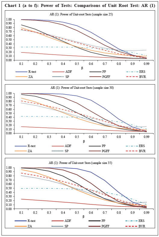
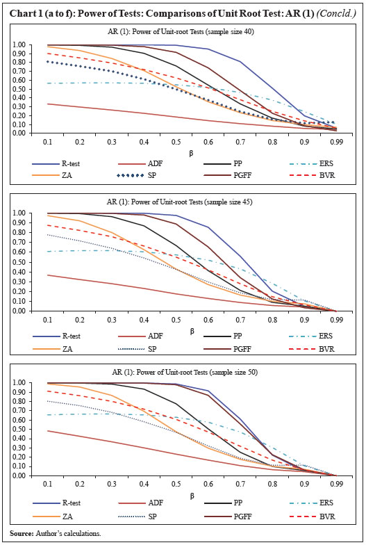
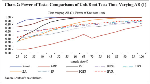 It is observed that the power or the ability to correctly identify a stationary series is significantly higher for the new test than for the other selected unit-root tests when the sample size is under 50. For large sample sizes, the new unit-root test mirrors either improved or on-par efficiency as compared to the other tests. Section V
Conclusions A new test criterion is developed in this paper to test the presence of unit root in a zero-mean time series with no deterministic trend and no structural break. The test statistic has been developed with the assumption that if a given data series is generated out of a random walk process, then it will result in a better fit when the PDF of a random walk process is applied to it, rather than force-fitting it with the PDF of a stationary process. The proposed unit-root test is generic in nature and is effective to any time series irrespective of the practitioner’s assumption on the time-variant coefficients or orders of AR/MA processes. To estimate the empirical PDF and critical values of the test statistic, the MCS method is used, wherein a large set (10 million) of known non-stationary series of various sample sizes (ranging from 20 to 100) are generated. The test statistic is then calculated for the generated data series, and is used as a reference. The performance of the proposed new unit-root test statistic is empirically compared with other commonly used univariate unit-root tests viz., ADF test, PP test, KPSS test ERS test, Zivot and Andrews test, Schmidt and Phillips (SP) test, PGFF test, and BVR test. For this purpose, all these selected unit root tests are applied individually to a large set of stationary as well as non-stationary data of varied length, which are synthetically generated using time-varying as well as fixed AR(1) and AR(2) models for stationary data, and random walk model for non-stationary data. It is observed that for small samples, the power of the proposed test is significantly higher than the other selected unit-root tests, particularly when the sample size is under 50. For large samples, the effectiveness of the proposed test is still higher than most of the selected tests and is on-par with the remaining ones. The higher power of the test is demonstrated only under the case of no trend and no structural breaks. However, most of the time series data have trends, which bring in another source of non-stationarity. The proposed test can be developed further to account for the trend and structural breaks. Further, although the new test demonstrates improved performance when error terms are correlated, the specific design and derivation of the PDF of the test statistic with correlated error terms is another area for future work. References Breitung, J. (2002). Nonparametric tests for unit roots and cointegration. Journal of econometrics, 108(2), 343-363. C. R. Rao. (2009). Linear Statistical Inference and its applications, 2nd edition. Dickey, D. A., and W. A. Fuller (1979). Distribution of the Estimators Time Series With a Unit Root, Journal of the American Statistical Association. Dickey, D. A., and W. A. (1981). Likelihood Ratio Statistics for Autoregressive Time Series With a Unit Root, Econometrica, 49,1057-1072. Elliott, G., T. J. Rothenberg, and J. H. Stock. (1996). Efficient Tests for an Autoregressive Unit Root, Econometrica, 64, 813-836. Fuller, W. A. (1996). Introduction to Statistical Time Series, New York: Wiley Jansson, M., Nielsen, M.Ø., (2012). Nearly efficient likelihood tests of the unit root hypothesis, Econometrica, 80, 2321–2332. Kwiatkowski, D., P.C.B. Phillips, P. Schmidt, Y. Shin (1992). Testing the Null Hypothesis of Stationarity against the Alternative of a Unit Root, Journal of Econometrics, 54:159-178, North-Holland. MacKinnon, J. G. (1991). Critical Values for Cointegration Tests. In Engle, R. F., Granger, C. W. J. (Eds.), Long Run Economic Relationships. Oxford University Press (pp. 267–276). Pantula, S. G., G. Gonzalez-Farias, and W. A. Fuller (1994). A comparison of unit-root test criteria, Journal of Business & Economic Statistics 12 (4), 449-459. Pesaran, M. H. (2015). Time Series and Panel Data Econometrics. Oxford University Press. Phillips, P. C. B., Perron, P. (1988). Testing for a unit root in a time series regression, Biometrika, 75 (2): 335–346. Schmidt, P. and Phillips, P.C.B. (1992). LM Test for a Unit Root in the Presence of Deterministic Trends. Oxford Bulletin of Economics and Statistics, 54(3), 257–287. Skrobotov, A. (2018). On bootstrap implementation of likelihood ratio test for a unit root, Economics Letters 171, 154–158. Solberger, M. (2013). Likelihood-Based Tests for Common and Idiosyncratic Unit Roots in the Exact Factor Model. Acta Universitatis Upsaliensis. Digital Comprehensive Summaries of Uppsala Dissertations from the Faculty of Social Sciences, 90: 51, Uppsala. Zivot, E., and Andrews, D. (1992). Further evidence on the great crash, the oil -price shock, and the unit-root hypothesis, Journal of Business & Economic Statistics, 10(3): 251-270.
Annex
|