Monetary Policy Transmission and Labour Markets in India

By

Chetan Ghate
Satadru Das
Debojyoti Mazumder
Sreerupa Sengupta
Satyarth Singh^*

Abstract

How does informality in labour markets affect inflation stabilisation and monetary policy setting by central banks? To address this, we build a medium-scale NK-DSGE model with segmented labour markets. We introduce search and matching frictions in both formal jobs as well as in informal casual jobs. We calibrate the model to India. As in the data, our model is able to replicate the impact of a contractionary monetary policy shock on lower output and inflation via higher formal and informal unemployment. As a counterfactual exercise, when we increase the magnitude of formality, we show that the impact of a contractionary monetary policy shock leads to a larger impact on inflation, suggesting that monetary policy transmission improves.

JEL Codes: E52, E24, E26, E32, E63, E61

Keywords: Business cycles, informal labour markets, monetary policy transmission, inflation targeting, monetary fiscal coordination, NK-DSGE models

Acknowledgement

The authors are grateful to the Reserve Bank of India (RBI) for supporting the study through its DRG Studies Series. The views expressed here are those of the authors and not of the organisations to which they belong. The authors are grateful to Smt. V. Dhanya, Shri Gautam Kumar Das, participants of the 6th Asia KLEMS Conference held in Lonavala in June 2023, participants of the DEPR Study Circle seminar, and an anonymous referee for comments. They are grateful to Subhadeep Halder for outstanding research assistance. All remaining errors and omissions are the authors’ responsibility.

Chetan Ghate
Satadru Das
Debojyoti Mazumder
Sreerupa Sengupta
Satyarth Singh

Executive Summary

A large literature on emerging market and developing economies (EMDEs) using the Dynamic Stochastic General Equilibrium (DSGE) models highlight the importance of informal labour markets in shaping business cycles. While DSGE models are increasingly being used to study business cycles in the Indian economy, many of these models are constructed without reference to labour markets because of the lack of a comprehensive data set on formal and informal labour market indicators.

The key research question this study addresses is what implications labour market informality has for inflation stabilisation and monetary policy transmission under an inflation targeting regime. The study builds a New Keynesian Dynamic Stochastic General Equilibrium (NK-DSGE) model with formal and informal labour markets to address this question. While the model is calibrated to India, the NK-DSGE setup is general enough to study monetary policy transmission in countries with large informal labour markets.

The study makes several contributions. First, it uses the annual India KLEMS dataset with additional information from the National Sample Survey (NSS), Periodic Labour Force Survey (PLFS) datasets to identify key labour market stylised facts that characterise the business cycle in India over a 40-year period. The study finds regular (formal) employment to be pro-cyclical. Casual employment (informal), in contrast, is counter-cyclical. Self-employment, which constitutes the bulk of informal employment, has an insignificant correlation with output. This suggests that upturns in the Indian business cycle have historically been associated with an increase in regular (formal) employment, and a decline in casual (informal) employment.

The India KLEMS dataset is available only at an annual frequency. To study the impact of monetary policy shocks at a higher (monthly) frequency, the study assembles a high frequency monthly data using the Consumer Pyramids Household Survey (CPHS) dataset compiled by CMIE. The CPHS reports employed workers under four categories: business, salaried employees, small traders and wage labourers, and farmers. These provide broad proxies for formal and informal employment in the economy. Using the CPHS data, our study uses a Local Projections (LP) framework to identify the impact of a monetary policy shock on a handful of key macroeconomic variables. The study finds that a contractionary monetary policy leads to a decline in inflation and a decline in growth after a lag.

To capture the stylised facts and the Impulse Response Functions (IRFs) from the KLEMS and CPHS datasets, the study builds a NK-DSGE model with dual labour markets and search and matching frictions. The model is calibrated to India. The study assumes that the labour market is segmented between formal and informal labourers in line with the literature describing the labour market of emerging economies. The formal sector has both public and private sector jobs that are subject to search and matching frictions. In the informal sector, there is self-employment and casual jobs, although only casual jobs are subject to search and matching frictions. Using this framework, the study examines the implications of informality for inflation stabilisation and monetary policy under the inflation targeting regime.

As in the data, the study finds that a contractionary monetary policy shock leads to a decline in aggregate consumption, decline in inflation, decline in investment, a decline in output, a decline in the capital stock, and a decline in private formal employment. Unemployment rises in both formal and informal labour markets. There is a decline in casual and self-employment, which leads to total informal employment falling. When there is an increase in the proportion of formal firms contributing to final goods production (3 per cent relative to baseline), a contractionary monetary policy shock leads to a small additional reduction in inflation relative to baseline on impact. This suggests that monetary policy is more effective when there is a higher degree of formality in the economy.

In sum, the study provides a conceptual framework to understand the mechanism behind monetary policy transmission in an emerging market economy with a diverse labour market, like India. The study shows that formality in the labour market affects the impact of monetary policy shocks on inflation and other macroeconomic variables. The study shows that monetary policy transmission under inflation targeting improves with more formality in the labour market.

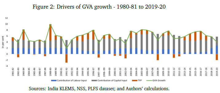
1 Introduction

A large literature on emerging market and developing economies (EMDEs) using Dynamic Stochastic General Equilibrium (DSGE) models highlights the importance of informal labour markets in shaping business cycles.¹ While DSGE models are increasingly being used to study business cycles in the Indian economy (Gabriel et al., 2012, 2016; Ghate et al., 2018; Banerjee and Basu, 2019; Banerjee et al., 2020; Kumar, 2023), many of these models are constructed without reference to labour markets because of the lack of a comprehensive data set on formal and informal labour market indicators.²

The key research question this study addresses is what implications labour market informality has for inflation stabilisation and monetary policy transmission under inflation targeting regimes. The novel aspect of our study is that we build a NK-DSGE model with formal and informal labour markets to address this question. While our model is calibrated to India, our NK-DSGE setup is general enough to study monetary policy transmission in countries with large informal labour markets. The India KLEMS dataset provides an annual time series of persons employed. The KLEMS database with additional information from the National Sample Survey (NSS) and Periodic Labour Force Survey (PLFS) datasets further allows us to calculate the composition of total employment between regular workers (formal), and casual and self-employed workers (informal).³ Figure 1 depicts formal and informal employment trends in the Indian economy between 1980-81 and 2019-20. Informal employment consists of self-employed and casual workers whereas formal employment consists of regular workers.⁴ Figure 1 shows that self-employment dominates the total employment structure. Over time, however, its share has declined very slowly from 58 per cent in 1980-81 to 53 per cent in 2019-20.⁵ Casual workers constituted about 29 per cent of employment in 1980-81, which declined to 23 per cent during 2019-20. The share of informal employment (self-employment and casual) has declined very slowly over the years, and constitutes the bulk of employment today. Formal employment has increased from 13 per cent in 1980-81 to 24 per cent during 2019-20. This is primarily driven by the formalisation of workers in the manufacturing sector where the share of regular employment has increased from 27 per cent in 1980-81 to 50 per cent in 2019-20.

Figure 2 presents a growth accounting decomposition, where real gross value added (GVA) growth is decomposed between contributions from factor accumulation (labour and capital) and total factor productivity (TFP) growth. The long-term drivers of GVA growth show that during 1980-81 and 2019-20, the capital input is the dominant factor (64.9 per cent average) over the sample period. The labour input plays a significant role and on average accounts for 31.5 per cent of GVA growth. The remaining 3.6 per cent of GVA growth is explained by growth in total factor productivity.⁶

The India KLEMS dataset is available only at an annual frequency. To study the impact of monetary policy shocks at a higher (monthly) frequency, we assemble a high frequency monthly data using the Consumer Pyramids Household Survey (CPHS) dataset compiled by CMIE.⁷ The CPHS reports employed workers under four categories: business, salaried employees, small traders and wage labourers, and farmers. These provide broad proxies for formal and informal employment in the economy. Using the CPHS data, we use a local projections (LP) framework to identify the impact of a monetary policy shock on a handful of key macroeconomic variables.⁸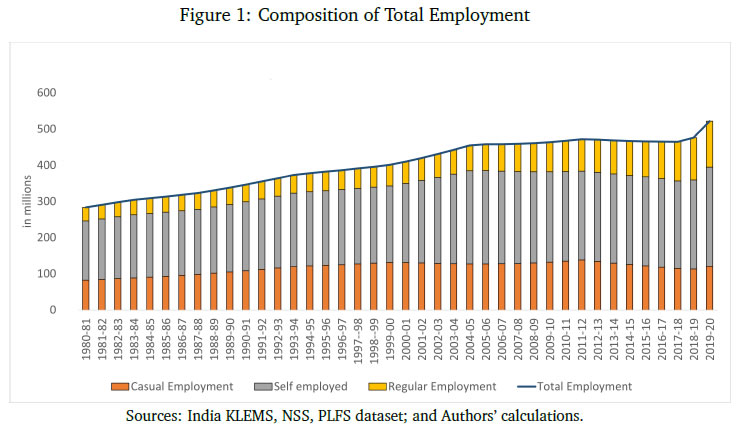

Using the CPHS dataset, we generate impulse response functions (IRFs) that characterise the impact of monetary policy shocks on several macroeconomic variables. We find that a one standard deviation contractionary shock in monetary policy leads to a small negative effect on the unemployment rate (unemployment falls) in the first 12 months after the shock, but the effect turns positive (unemployment rises) for up to 36 months after the shock, although the shock estimates are mostly not significant. In the case of CPI Inflation (Industrial workers), inflation declines and the effect is statistically significant for up to 20 months after the shock. Growth, proxied by a nine-indicator dynamic factor model using nine high frequency indicators, rises initially, and then falls after 15 months, and remains negative for up to 32 months after the shock. Contractionary monetary policy, therefore, leads to a decline in inflation, a rise in unemployment after a lag, and a decline in growth after a lag.

Our study makes several contributions. First, we use the annual India KLEMS, NSS, PLFS dataset to identify key labour market stylised facts that characterise the business cycle in India, a large emerging market economy over a 40 year period. We find regular (formal) employment to be pro-cyclical. Casual employment (informal), in contrast, is counter-cyclical.⁹ Self-employment, which constitutes the bulk of informal employment, has an insignificant correlation with output. This suggests that upturns in the Indian business cycle have historically been associated with an increase in regular (formal) employment, and a decline in casual (informal) employment. These results also hold when we confine output to ';modern sector'; output by combining manufacturing and service sector GVA to get modern sector GVA.¹⁰

To capture the stylised facts and the IRFs from the KLEMS and CPHS datasets, we build a NK-DSGE model with dual labour markets and search and matching frictions. We calibrate the model to India. We assume that the labour market is segmented between formal and informal labourers in line with the literature describing labour market of emerging economies (Gutierrez et al., 2019; Sugiharti et al., 2022). The formal sector has both public and private sector jobs which are subject to search and matching frictions. In the informal sector, there are self-employment and casual jobs. We assume that only casual jobs in the informal sector are subject to search and matching frictions. Like Michaillat (2014), households derive utility over consuming a final private good and a public good. The final private good is produced by two types of intermediate goods firms: formal intermediate good firms and informal intermediate good firms. The public good is produced only by formal labour.

Both formal firms and the government look for workers by posting vacancies, and only a fraction of vacancies are matched. Firms in the informal sector looking for casual workers also post vacancies. Unemployed workers search for jobs. Wages are determined by Nash wage bargaining, where casual labour has less bargaining power. Labour market segmentation means that households either supply hours in the formal sector, or in the informal sector. Monetary policy follows a Taylor Rule. Like Alberola and Urrutia (2020), we are interested in the implications of informality for inflation stabilisation and monetary policy under inflation targeting regimes. Our model incorporates features of both Michaillat (2014), and Alberola and Urrutia (2020). We extend the analysis in Michaillat (2014) by adding informality to his model.

We find that a contractionary monetary policy shock leads to a decline in aggregate consumption, decline in inflation, decline in investment, a decline in output, a decline in the capital stock, and a decline in private formal employment. Unemployment rises in both formal and informal labour markets. There is a decline in casual and self-employment which implies that total informal employment falls. When we exogenously raise the proportion of formal firms contributing to final good production (3 per cent relative to baseline), we find that a contractionary monetary policy shock leads to a small additional reduction in inflation relative to baseline on impact, suggesting that monetary policy is more effective when there is more formality in the economy. When we conduct a counterfactual analysis using a higher increase in the formal good elasticity with respect to output, we get a reduction in the impact effect of monetary policy relative to baseline.

2 Stylised Facts

2.1 GVA and Employment: KLEMS, NSS and PLFS Datasets

Real gross value added (GVA), regular, casual and self-employment series for India for the period starting 1980-81 to 2019-20 are obtained from India KLEMS data with additional information from NSS and PLFS employment-unemployment survey rounds.¹¹ We choose real gross value added (GVA), real gross domestic product (RGDP), regular, casual, and self-employment (in numbers of people) and interest rates as our key variables. The cyclical components of GVA, RGDP, and the employment series are extracted using a full sample, asymmetric Christiano-Fitzgerald (CF) filter after removing a linear trend.¹² The cyclical components of the variables are then used for correlations, standard deviations, relative standard deviations and the co-variance. The detailed data source of the variables and the transformations used are provided in Appendix A. We generate stylised facts for employment and output cycles for three alternate specifications - (i) total GVA, (ii) modern sector GVA, and (iii) modern sector plus construction GVA. This allows us to study how formal and informal employment have varied across the Indian Business Cycle over the last 40 years, and how these relationships differ across broad sectors in the economy.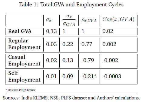

Figure 3 plots the cyclical component of regular employment (formal), casual employment (informal), and self-employment (informal) with respect to total output (measured using GVA). Table 1 and Figure 3 show that during a business cycle upturn, an increase in output increases the demand for regular employment, whereas during an economic downturn, due to less employment opportunities and the relatively higher wages of formal workers, regular employment decreases. Casual employment and GVA cycles on the other hand are counter-cyclical. During a business cycle downturn there is an increase in the employment of casual workers as firms switch demand from workers in regular employment to casual employment. During a business cycle upturn, due to increased demand, firms tend to hire more regular workers with higher skills and hence the demand for casual workers goes down and the demand for regular workers increases.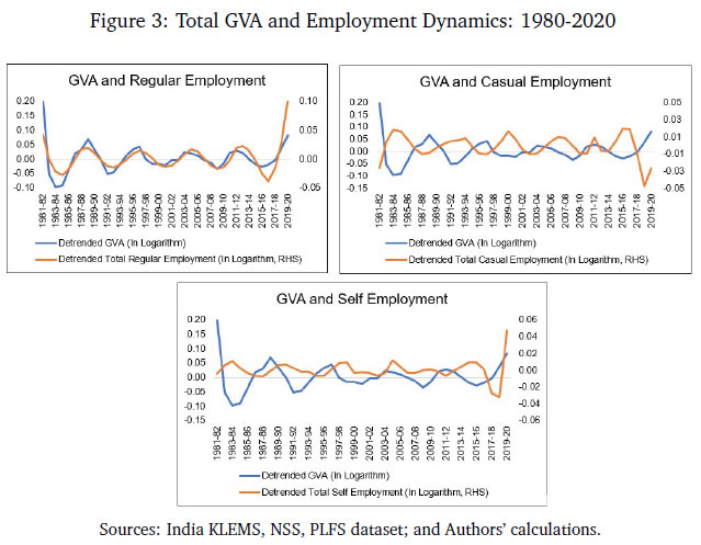

When we re-do the above exercise by adding manufacturing and service sectors to get ';modern sector'; GVA, the results strengthen. As can be seen from Table 2, the covariance between regular employment and GVA is positive (0.01). Formal employment is pro-cyclical when output is measured by modern sector GVA. In contrast, the covariance between casual employment and GVA is −0.01, or counter-cyclical. The correlation between self-employment and modern sector GVA is statistically insignificant like before.¹³ Modern sector GVA and employment cycles are shown in Figure 4.¹⁴

Finally, to study employment over changing structural pattern of the economy we examine the business cycle moments across three sub-periods: 1980-81 to 1999-00, 2000-01 to 2009-10 and 2010-11 to 2019-20. The results show that the volatility of real GVA and regular employment is 0.18 and 0.03, respectively, during 1980-81 to 1999-00, and this declines to 0.02 and 0.01, respectively, between 2000-01 to 2009-10, but further increases to 0.03 and 0.04, respectively, during 2010-11 to 2019-20.

Employment relative to output has witnessed an increased volatility over the years. During 2010-11 to 2019-20 regular employment was 1.2 times more volatile than real GVA.¹⁵

2.2 Empirical Impulse Response: CPHS Dataset

To supplement the stylised facts from Sub-section 2.1 with IRF analysis, we assemble high frequency monthly data on various macroeconomic and macro-financial indicators. These include overnight indexed swap (OIS) rates, interest rates of various terms, monthly price inflation, a multi-variable monthly economic activity indicator, and monthly unemployment rate from the CPHS dataset compiled by CMIE. The data for the interest rates, OIS, economic activity, and inflation are from the period January 2010 to November 2019, while for the unemployment the data is only available from January 2016 and runs up to November 2019.¹⁶ Using this data, we use a local projections (LP) framework to identify the impact of a monetary policy shock on a variety of macroeconomic variables including labour market indicators. Specifically, we estimate the following set of regressions.

In the model above, X is a macroeconomic or macro-financial outcome variable, and ee_t−1 is the measure of the monetary policy shock. The coefficients β_h are plotted against time to obtain the impulse response functions (IRF) along with their confidence interval bands. The outcome variables analysed in this model are short-term and long-term sovereign bonds, inflation rate as measured by consumer price index - industrial workers (CPI-IW) and wholesale price index (WPI), a high frequency fifteen indicator dynamic factor measure of economic activity which has been shown to track year-on-year, quarterly GDP growth rate well (Bhadury et al., 2021), and the seasonally adjusted unemployment rate obtained from the CMIE. The level series of the economic activity indicator is seasonally adjusted, log-transformed and de-trended using an assymetric Christiano Fitzgerald filter to obtain the cycles. The local linear projections are carried out on these cycles.

The measure of the monetary shock is calculated using a methodology similar to Coibion et al. (2019). They use the movement of federal funds futures immediately after the announcement of monetary policy to calculate the unanticipated component of monetary policy. This strategy helps in filtering out the components of monetary policy which are in response to prevailing macroeconomic conditions and therefore already priced into future contracts. Therefore, the movement in the prices of futures contracts immediately after the policy should represent innovations in the policy. However, in the case of India, there are no marketable futures contract on the policy rate. To bypass this issue, the one-day change in the yield of one month overnight indexed swap (OIS) contracts on the day of the policy is used as the measure of monetary policy surprise or innovation. The one-day change in yields of OIS contracts in India has been found to capture monetary policy or other macroeconomic shocks adequately; it has also been found to be an effective predictor of market reaction to monetary policy shocks (Das et al., 2020). In the present study, the monthly average of shocks is used as the main explanatory variable.¹⁷

The sample is restricted between January 2010 and November 2019 for the following reasons: first, the measure of the monetary policy shock, i.e., OIS data, is not available for all days prior to 2010. Second, the RBI undertook several unconventional monetary policy actions apart from changes in the policy rate from November 2019 which will complicate the relationship between OIS and the policy rate. Third, the study intends to avoid the COVID period.

The results from the empirical exercise are represented in terms of the following IRFs in Figure 5. The black line plots the reaction of the macro variables to one standard deviation shock in monetary policy. The darker shaded region is a one standard deviation confidence interval, and the lighter shaded region is 2.0 times the standard deviation confidence interval. The reaction of the 90-day T-Bill and 10-year government security (GSEC) should be interpreted in terms of per cent, that of inflation are to be interpreted in terms of basis points, and that of the economic activity index to be interpreted in terms of percentage points. The standard deviations are obtained using Newey-West standard errors to make them robust to serial auto-correlation.

The first and second panel shows the effect of one standard deviation shock in monetary policy on short-term (T-Bill rates) and long-term government securities (10-year GSEC yield). The IRFs show that the effects are positive and immediate, and remain statistically significant for up to 25 months after the shock for T-Bills and up to 16 months for GSECs. The third and fourth panel shows the reaction of inflation to the same shock. In case of inflation in CPI-IW, the effect is statistically significant and negative from 4 months after the shock and remains negative and significant for up to 20 months from the shock. The reaction of WPI based inflation is delayed, and is negative and significant from twelve months after the shock to up to 25 months. The fifth panel shows the effect on output cycles as captured by the de-trended fifteen indicator dynamic factor. The effect is negative and significant from 3 months after the shock and largely remains in the negative region up to 20 months after the shock, although statistically not always significant.¹⁸ The unemployment data at monthly frequency is only available from 2016, leading to few number of observations. As a result, the local linear projections provide imprecise estimates of impulse response with high volatility and statistically insignificant coefficients. However, directionally the IRF shows a fall in unemployment rate on impact which increases and becomes positive after 10 quarters. The IRF for unemployment rate is not reported for their impreciseness.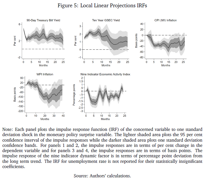

3 The Model

From Section 2.1, it is apparent that the relation between the GVA cycle and the employment cycle of different types of employment are varied. This suggests segmentation in the labour market. How does an economy with segmented labour markets react to a monetary policy shock? In this section we try to answer this question by building a medium scale NK-DSGE model with dual labour markets. We calibrate the model to match moments of the modern sector of the Indian economy as presented in Table 2.¹⁹ We use this model, which corroborates broadly with the salient features of the Indian economy, to understand the effect of a monetary policy shock on different types of employment. We show that the direction of the model generated impulse response for relevant variables are largely in line with the empirically estimated impulses, estimated in Section 2.1. We also study the outcomes from the monetary policy shock under different counterfactual scenarios by exploiting the baseline model framework.

Our model features both formal private and public sector jobs, and casual and self-employment in the informal sector. The labour market is assumed to be segmented between formal and informal labourers, as in Srivastava (2019). Labour market segmentation means that households either supply hours in the formal sector, or in the informal sector. We calibrate the model to India. We target six parameters, which we match precisely in the model. We also target two other parameters which we match reasonably well, suggesting reasonably good model validation.

3.1 Final Good Production

The private final good, p, is produced by two types of monopolistically competitive intermediate good firms: formal intermediate good firms and informal intermediate good firms. The public good, g, is produced by formal labour, employed in the public sector (L_g,t). For simplicity, we assume that formal and informal intermediate goods are produced by ϕ and 1 − ϕ measures of monopolitically competitive firms, respectively. Formal firms are indexed by i and informal firms are indexed as j. The production function of final good bundles formal (Y_F) and informal (Y_I) intermediate goods as follows,

3.2 Labour Markets

Labour dynamics of formal sector workers and casual workers can now be defined. Employment dynamics in the frictional labour markets has two parts: workers who retain their jobs and workers who are newly employed from the unemployed pool. For the formal sector, the labour dynamics which a household faces are given by

Similarly, for casual labour in the informal sector the dynamics are given by,

The total number of casual labour at time t is the total of the number of casual workers who retain their jobs from last period and the number of newly employed casual workers matched from the unemployed pool of informal labourers.

3.3 Households

Following Alberola and Urrutia (2020), an infinitely lived household has both formal and informal types. We assume that the formal (F ) and informal (I) sectors have employment that are of two types each. Households derive utility from consuming the final private good and a public good. The household’s expected utility function follows Michaillat (2014), and is given by

The household budget constraint is

The FOC with respect to public sector’s formal labour supply is given by equation (24):

3.4 Profits and Wages

We now describe the formal and informal firm’s profit maximisation and wage determination problems. We provide details of the derivations in Appendix D.2.1 and D.2.2.

3.4.1 Profit Maximisation

The discounted sum of the infinite profit stream for formal firms (indexed by i) are given by

Equation (35) shows that on the margin, the return from self-employed labour (LHS) is equal to the wage cost (RHS). Since, the self-employed labour market does not have a search and matching friction, the net shadow price term does not appear in equation (35).

3.4.2 Wage Determination

The standard Nash sharing rules from equation (38) and equation (39) are given by

3.5 Government

3.6 Monetary Policy

3.7 Market Clearing

After incorporating the firms’ per period profit and the government’s budget constraint into the household’s budget constraint, the economy-wide resource constraint is obtained. The price of the formal sector intermediate good is assumed to be the numeraire.

Final goods production is used to consume (adjusted for Rotemberg pricing), invest, and to pay the fixed costs of posting vacancies, by both formal and informal firms.

3.8 New Keynesian Phillips Curve

The NKPC is similar in form to that in Michaillat (2014). The NKPC equates current inflation, to future expected inflation, and a composite term corresponding to output (which includes the terms of trade).

4 The Quantitative Model

The primary focus of our study is to use the model to compute outcomes of the endogenous variables in the economy under a monetary policy shock with varying degrees of formality. We calibrate the model to India.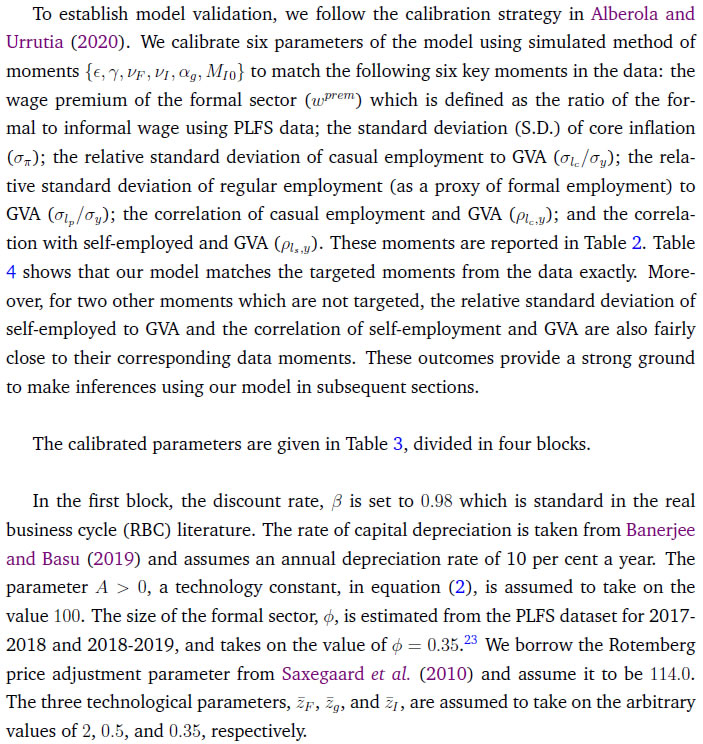

In the second block, the parameters correspond to the labour market block of the model. The wage income tax, τ, proxies for the share of direct (labour) income taxes as a percentage of GDP, which is approximately 2.5 per cent as of 2022. Both the job loss rate of the formal private sector and the public sector are obtained from Das et al. (2023).²⁴ As can be seen, the rate of job loss in the private sector is greater than the job loss rate in the public sector. The matching elasticity of the formal sector η_F and η_I are taken from Alberola and Urrutia (2020) and set to 0.4. We borrow the value of χ_F = 0.71 and χ_g = 0.21 from Alberola and Urrutia (2020) and Michaillat (2014) to proxy for the cost of posting vacancies in the private and public formal sectors. The labour income share of private formal income, α_F = 0.64, is estimated from the national accounts data, where the labour income share is estimated as a ratio of compensation of employees to GVA of private corporations. The job loss rate of the casual sector is estimated from the PLFS 2017-2018, 2018-2019, to be 0.05.²⁵ The cost of posting a vacancy for casual labour, χ_I, is borrowed from Michaillat (2014), and estimated to be 0.21.

The casual labour income share, α_I is estimated from the CPHS data published from CMIE in the following way: first, the aggregate quarterly earnings of all workers identified as ';casual worker'; in the dataset is averaged over quarters; next, the average aggregate quarterly earnings of all workers in the informal sector is similarly calculated; and lastly, α_I is obtained as the ratio of the two. It is assumed that since the informal sector utilises very little or no capital, all the factor income in the sector is distributed as labour earnings, thereby making aggregate labour income of the informal sector as a measure of the sector’s GVA. The value obtained for α_I is 0.19.

In the third block, the parameters correspond to the Taylor Rule in equation (46), which are borrowed from the recent macro literature on India.

5 Inspecting the Mechanism in the Baseline Model

We consider the impact of a one standard deviation contractionary monetary policy shock on the economy in a variety of environments which may be relevant to the Indian economy (higher formality, higher public sector wages) and other emerging market economies. We first, however, understand the mechanism behind how monetary policy transmits in the baseline model. These impulse response functions are given in Figures 6a, 6b and 6c.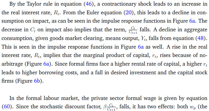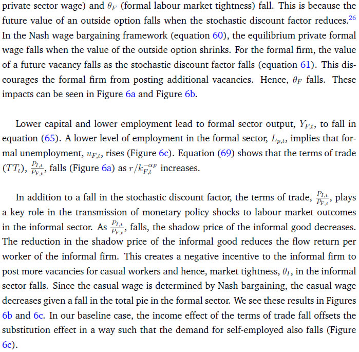

Hence, a contractionary monetary policy shock on impact leads to a decline in aggregate consumption, decline in inflation, a decline in output, a decline in the capital stock, and a decline in private formal employment. Unemployment rises in both formal and informal labour markets, while both casual and self-employment fall. The model generated impulse response functions are broadly consistent with the impulse response functions in Figure 5, where a monetary policy shock leads to lower inflation and lower output, via higher unemployment in both formal and informal labour markets.

6 Counterfactual Analysis

We study the impact of a contractionary monetary policy shock in three environments. We compare the impact with the baseline for changes in formality, ϕ, a change in the public sector, w_g, and a change in the formal input elasticity with respect to output, γ. The first experiment proxies for higher formality in the economy. The second experiment assesses the general equilibrium effects of periodic revisions in public sector wages enacted by many developing countries, including India. The third experiment is also a proxy for more formality in the economy.

6.1 Increase in the size of the formal sector

The impact of a contractionary monetary policy with higher ϕ is given in Figures 7a, 7b and 7c. We assume that the size of the formal sector (proxied by ϕ) increases by 3 per cent from its baseline level specified in Table 3. The change in the size of the formal sector is a slow moving variable in a country like India.

Relative to baseline, inflation witnesses a small additional reduction given the small increase in the size of formal sector (from the NKPC in equation 49). Monetary policy therefore transmits better and is more impactful. However, there are differentiated sectoral effects compared to baseline. The relative demand for the informal good to produce the final good reduces because of a higher ϕ. That induces an additional negative effect on job creation in informal labour compared to baseline. This leads to an additional fall in market tightness in the labour market of the informal sector over and above baseline. This causes an additional reduction in both the casual wage, w_c, and the self-employment wage, w_s, compared to baseline. However, the relative fall in w_s is larger than w_c which encourages informal firms to substitute casual worker with self-employed. Thus, the employment of casual labour decreases further, but the employment of self-employment increases. This is in contrast to the baseline, where both casual and self-employment fall in response to a contractionary monetary policy shock. The insight we gain from this exercise is that when there is a contractionary monetary policy shock, higher formality induces a change in the composition of informal employment, away from casual employment, and towards higher self-employment. Output, consumption, employment, fall as in the baseline. Informal unemployment and formal output are more volatile.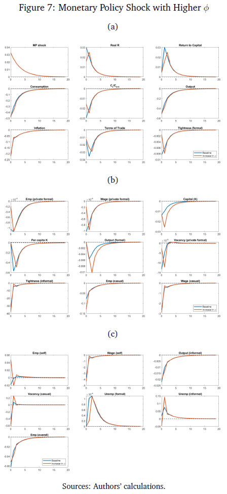

6.2 Increase in the public sector wage

Emerging market and developing economy formal labour markets have a high public sector presence (Ghate and Mazumder, 2019). We now examine how a contractionary monetary policy shock interacts with an increase in the public sector wage by 23 per cent, the most recent public sector pay increases instituted in 2015 in India, as part of the Seventh Pay Commission (Figures 8a-8c).²⁷

6.3 Increase in the formal good elasticity of output

In our model, a one per cent increase in the use of the formal good as an input translates to γ percentage increase in final output - the formal good elasticity with respect to output. The parameter γ is estimated in Table 3 of Section 4 to match the target variables from the data. Figures 9a, 9b and 9c show the effect of contractionary monetary policy shock on the economy when γ is (arbitrarily) one and half times greater than its baseline value in Table 3.

As in the case of a higher ϕ, a higher value of γ does not have much of an impact by the monetary policy shock on final good and consumption. The impact of a contractionary monetary policy shock is however seen more at the sectoral level. In the informal sector, a higher γ moderates the fall in market tightness (equation 37) and that results in a moderated fall in the wage of casual and self-employed workers (equations 71 and 72). A higher γ makes a monetary policy shock more contractionary for private formal employment, wage and the capital stock. However, differentiated relative wage changes in the informal sector impacts the demand for casual workers in a way where casual employment increases and self-employment falls compared to baseline. Unlike a higher ϕ, a contractionary monetary policy shock reduces the impact of monetary policy on inflation relative to baseline. That leads to a further increase in the real interest rate. As a result, the stochastic discount factor falls more than the baseline level. That leads to additional reduction in the formal sector wage and market tightness. Thus, we see a further reduction in formal employment compared to the baseline.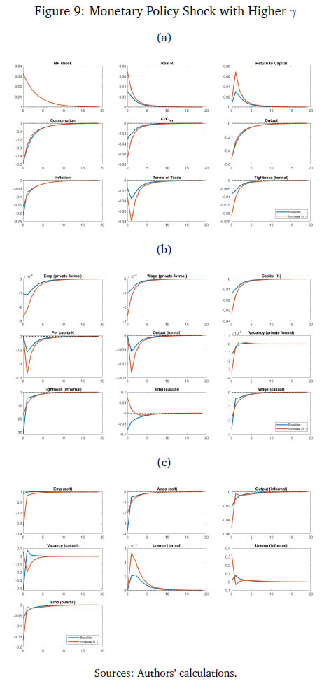

7 Conclusion

A central concern of macro stabilisation policy is to devise fiscal and monetary policies that influence the prospects for growth and mitigate the distress due to business cycle fluctuations. A proper evaluation of the benefits of stabilisation policy however requires knowledge of the determinants of growth and business cycles (Fisher et al., 1999). Our study provides new insights into the transmission of monetary policy in emerging market and developing economy labour markets. We make several contributions. First, we identify a set of stylised facts on how different types of employment (formal, informal) vary across the Indian business cycle using the annual data based on employment un-employment survey rounds by NSS, PLFS and the India KLEMS dataset from 1980-81 to 2019-20. We find that while regular employment is pro-cyclical, casual employment is counter-cyclical historically. To the best of our knowledge, this is the first rigorous analysis using annual employment data (constructed using information from NSS, PLFS and India KLEMS datasets) to identify a set of stylised facts of India’s labour market indicators. We also augment our empirical analysis with high-frequency monthly data from the CPHS dataset to generate IRFs using local projections that quantify the impact of monetary policy shocks on inflation, the unemployment rate, and output.

Building on Michaillat (2014) and Alberola and Urrutia (2020), we construct a NK-DSGE model with dual labour markets and search and matching frictions to replicate the IRFs. We assume that the labour market is segmented between formal and informal labourers. While our model is calibrated to India, our NK-DSGE setup is general enough to study monetary policy transmission in countries where there are large informal labour markets.

We find that a contractionary monetary policy shock impacts both inflation and out-put negatively, as in the data. We find that a contractionary monetary policy shock leads to both a decline in formal and informal employment, and therefore total employment, and leads to lower market tightness in both the formal and informal sector. While the IRF for unemployment using local projections is inconclusive because of the lack of a long enough sample, in the calibrated model, monetary policy impacts unemployment in both informal and formal labour markets negatively. In a counter-factual experiment, when we exogenously raise the proportion of formal firms contributing to final good production (3 per cent relative to baseline), we find that a contractionary monetary policy shock leads to a small additional reduction in inflation relative to baseline on impact, suggesting that monetary policy is more effective when there is more formality in the economy.

Our study uncovers new insights governing the transmission of monetary policy via labour markets in a large emerging market economy like India.

References

Alberola, E. and Urrutia, C. (2020). Does informality facilitate inflation stability? Journal of Development Economics, 146:102505.

Auerbach, A. J. and Gorodnichenko, Y. (2013). Output spillovers from fiscal policy. American Economic Review, 103(3):141–146.

Banerjee, S. and Basu, P. (2019). Technology shocks and business cycles in india. Macroeconomic Dynamics, 23(5):1721–1756.

Banerjee, S., Basu, P., and Ghate, C. (2020). A monetary business cycle model for india. Economic Inquiry, 58(3):1362–1386.

Bhadury, S., Ghosh, S., and Kumar, P. (2021). Constructing a coincident economic indicator for india: How well does it track gross domestic product? Asian Development Review, 38(02):237–277.

Bhadury, S., Ghosh, S., and Mazumder, D. (2022). A horse race among the alternative taylor rule specifications. Economic & Political Weekly, 57(23):48.

Castillo, P., Montoro, C., et al. (2010). Monetary policy in the presence of informal labour markets, volume 9. Banco Central de Reserva del Perú.

Coibion, O., Gorodnichenko, Y., and Ulate, M. (2019). Is inflation just around the corner? the phillips curve and global inflationary pressures. AEA Papers and Proceedings, 109:465–469.

Das, S., Ghosh, S., Mazumder, D., and Tushavera, J. (2023). Impact of COVID-19 shock on a segmented labour market: Analysis using a unique panel dataset. MPRA Working Paper.

Das, S., Surti, J., and Tomar, S. (2020). Does inflation targeting help information transmission? Available at SSRN 3701541.

Fernández, A. and Meza, F. (2015). Informal employment and business cycles in emerging economies: The case of mexico. Review of Economic Dynamics, 18(2):381–405.

Fisher, J. D. et al. (1999). The new view of growth and business cycles. Economic Perspectives - Federal Reserve Bank of Chicago, 23:35–56.

Gabriel, V., Levine, P., Pearlman, J., and Yang, B. (2012). An Estimated DSGE Model of the Indian Economy. In The Oxford Handbook of the Indian Economy. Oxford University Press: New York. (Eds. Chetan Ghate).

Gabriel, V., Levine, P., and Yang, B. (2016). An Estimated DSGE Model of the Indian Economy. In Monetary Policy in India: A Modern Macroeconomic Perspective. Springer Verlag. (Eds. Chetan Ghate and Kenneth M Kletzer).

Ghate, C., Gopalakrishnan, P., and Tarafdar, S. (2016). Fiscal policy in an emerging market business cycle model. The Journal of Economic Asymmetries, 14:52–77.

Ghate, C., Gupta, S., and Mallick, D. (2018). Terms of trade shocks and monetary policy in india. Computational Economics, 51:75–121.

Ghate, C. and Kletzer, K. M. (2016). Monetary Policy in India: A Modern Macroeconomic Perspective. Springer. (Editors).

Ghate, C. and Mazumder, D. (2019). Employment targeting in a frictional labor market. Indian Growth and Development Review, 12(2):242–262.

Ghate, C., Pandey, R., and Patnaik, I. (2013). Has india emerged? business cycle stylized facts from a transitioning economy. Structural Change and Economic Dynamics, 24:157–172.

Gutierrez, I. A., Kumar, K. B., Mahmud, M., Munshi, F., and Nataraj, S. (2019). Transitions between informal and formal employment: results from a worker survey in bangladesh. IZA Journal of Development and Migration, 9(1):1–27.

Jordà, Ò. (2005). Estimation and inference of impulse responses by local projections. American Economic Review, 95(1):161–182.

Jordà, Ò. and Taylor, A. M. (2016). The time for austerity: estimating the average treatment effect of fiscal policy. The Economic Journal, 126(590):219–255.

Kumar, A. (2023). Financial market imperfections, informality and government spending multipliers. Journal of Development Economics, 163:103103.

Kuttner, K. N. (2001). Monetary policy surprises and interest rates: Evidence from the fed funds futures market. Journal of Monetary Economics, 47(3):523–544.

Lakdawala, A. and Sengupta, R. (2024). Measuring monetary policy shocks in emerging economies: Evidence from india. Journal of Money, Credit and Banking. In press.

Michaillat, P. (2014). A theory of countercyclical government multiplier. American Economic Journal: Macroeconomics, 6(1):190–217.

Ramey, V. A. and Zubairy, S. (2018). Government spending multipliers in good times and in bad: evidence from us historical data. Journal of Political Economy, 126(2):850–901.

Saxegaard, M. M., Anand, R., and Peiris, M. S. J. (2010). An estimated model with macrofinancial linkages for India. International Monetary Fund.

Srivastava, R. (2019). Emerging dynamics of labour market inequality in india: Migration, informality, segmentation and social discrimination. The Indian Journal of Labour Economics, 62:147–171.

Sugiharti, L., Aditina, N., and Padilla, M. A. E. (2022). Worker transition across formal and informal sectors: A panel data analysis in indonesia. Asian Economic and Financial Review, 12(11):923–937.

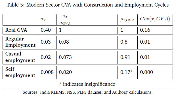
A Appendix

Gross Domestic Product: This study uses annual GDP data at constant prices for the total economy. The data is obtained from various rounds of NAS which are then spliced to convert the series to 2011-12 base prices. For tracking economic output (GDP) for the total economy on a monthly basis, a coincident economic indicator (CEII-9) representing all major sectors of the economy is used in the study.²⁸ The high frequency indicators used to construct monthly coincident economic indicator include IIP core, IIP consumer goods, auto sales, exports, non oil and non good imports, foreign tourist arrival, rail fright, air cargo and government revenue receipts. The method for constructing CEII-9 is adopted from Bhadury et al. (2021), and the high frequency indicators are obtained from the CEIC database.

Gross Value Added: This study also uses annual GVA data for the total economy and the modern sector. The National Accounts Statistics (NAS) published by NSO is the basic source of data for the annual GVA series. The total economy GVA includes value added for all sectors of economy namely agriculture, mining, manufacturing, construction, and services. The modern sector GVA data corresponds to gross value added of manufacturing and the service sector. The constant GVA series with base 2011-12 is used in the analysis.

Employment Data: We use PLFS and NSS Employment Unemployment survey rounds. For the annual employment series, the study uses data from the Employment Unemployment Survey rounds of the NSS 38th round (1983) to the 68th round (2011-12)) and the Periodic Labour Force Survey rounds (2017-18, 2018-19, 2019-20). The annual series of employment is constructed for the period 1980-81 to 2019-20 using the following steps:

Step 1: Worker participation rates (WPR) based on usual principal and subsidiary status are obtained from seven benchmark NSS rounds- 38th (1983-84), 43rd (1987-88), 50th (1993-94), 55th (1999-2000), 61st (2007-08), 66th (2009-10), and 68th (2011-12) rounds and three PLFS rounds (2017-18, 2018-19, 2019-20).

Step 2: The WPRs are applied to the census population to derive the total number of person employed for benchmark years. The data for the non-benchmark years are interpolated to create the time series of employment for 1980-81 to 2019-20.

Step 3: The total number of persons employed is further distributed to formal and informal workers. Formal workers include regular salaried workers and informal workers include casual and self-employed workers. Following PLFS classifications, regular workers are defined as workers who are working in other farm or non-farm enterprises as regular wage employees and correspond to PLFS activity status code 31. Casual workers are defined as workers who are engaged as casual wage labourer in public work and in other types of work and get a wage payment according to terms of daily or periodic work contracts (activity status code 41 and 51). The self-employed workers are defined as workers who are engaged in household enterprise as own account workers, employers and helpers (activity status code 11,12 and 21).

CMIE and Naukri Job Index database For quarterly and monthly employment series, data is obtained from Consumer Pyramid Household Survey ( CPHS) of CMIE database. Additional information on employment is also collected from Naukri JobS-peak Index.

The data source of CMIE data and Naukri JobSpeak Index are given as follows:

The CMIE employment series captures the estimated value of total number of workers employed under various categories of employment such as salaried employees, small traders and wage labourers, farmers, and business. The frequency of the data used in the study is March 2016 to December 2022 (Quarterly) and January 2016 to February 2023 (Monthly).

The Naukri JobSpeak published by Info Edge (India) Ltd. is a monthly Index representing the state of the Indian job market and hiring activity based on new job listings and job-related searches by recruiters on the resume database on Naukri.com. The JobSpeak Index captures hiring activity across multiple dimensions, including industries, cities, functional areas, and experience bands. The index is a reliable indicator of white-collar hiring in India. It is aggregated based on the hiring activity of over 100,000 clients with over 70 Lakh new job mandates yearly. The report does not cover gig employment, hyperlocal hiring, or campus placement. The frequency of the data used is July 2008 to December 2022.

Price Indicator: As an indicator of price the Wholesale Price Index data for 1990-91 to 2019-20 is obtained from the Office of Economic Adviser, Ministry of Commerce, Government of India. The WPI basket gives the highest weight to manufactured product (64.2 per cent), followed by primary articles (22.6 per cent) and fuel and power (13.2 per cent). The base year for WPI series is 2011-12. The WPI series of 1993-94 and 2004-05 are suitably linked to create the series from 1990-91 to 2010-11. From 2011-12 to 2019-20 the data is directly taken from WPI 2011-12 series.

Monetary policy Indicator: The weighted average call rate (WACR) is used as an indicator of monetary policy. The data is obtained from CEIC database. WACR is the volume weighted average of rates at which money at short notice (upto period of 14 days) are lent and borrowed in the money market. These rates can be computed for any period, daily, weekly and yearly. For this study, yearly WACR rates are used. The weighted average overnight call money rate was explicitly recognised as the operating target of monetary policy in 2011.

B Appendix

When we add construction GVA to modern sector GVA, we find that regular employment continues to be pro-cyclical (covariance = 0.01). Self-employment continues to be a-cyclical with respect to the real GVA cycle.²⁹ However, with the inclusion of construction, casual employment is now pro-cyclical (covariance = 0.01). The construction sector has emerged as the largest non-farm employment generator rising from 6.6 per cent of total employment in 1980-81 to 20.5 per cent of total employment in 2019-20. Further, casual workers, on an average, account for 76 per cent of employment in construction. When there is an upturn in the business cycle which typically leads to a boom in the construction sector, this leads to a greater demand for construction workers. As construction workers dominate the total pool of casual workers, this leads to the pro-cyclicality of casual employment and GVA. Table 5 summarises these results. Figure 10 plots the modern sector and construction GVA cycles against employment cycles.³⁰

C Appendix

As can be seen in Table 6, regular employment is significantly correlated with real GDP, and casual employment is significantly counter-cyclical. Self-employment is statistically a-cyclical with respect to GDP. All three types of employment are less volatile than output.

Figure 11 plots the cyclical component of regular, casual and self-employment with respect to output (measured using RGDP). During business cycle upturns, the demand for regular worker increases, where as casual workers declines and self-employment remains acyclical. Similarly, during a business cycle downturn, the employment of casual workers increases, and regular employment decreases as firms switch their demand of workers from regular to casual employment. This pattern is consistent when output is measured in terms of GVA.

D Appendix

D.1 Household Optimisation

D.2 Intermediate Goods

D.2.1 FOCs from the formal firms’ optimisation

D.2.2 FOCs from the informal firms’ optimisation

D.3 Wages

The formal private sector firms and workers negotiate the wage by the Nash bargaining rule. The rule is described in equation (38). Using equaiton(38) and the FOCs for {L_F,t} in the household optimisation and in the formal firms’ optimisation, equation (38) can be reworked as follows

Similarly, the wage of the casual worker is determined using equation (39) and the FOC for {L_c,t} in the household’s and in informal firms’ optimisation problem. That is,

E Appendix

The model block has 29 equations and 29 variables. The complete set of equations that we have used in our calibration are as follows:

Description of Variables

^* Chetan Ghate (cghate@isid.ac.in; cghate@iegindia.org) is the Director of the Institute of Economic Growth in New Delhi. Satadru Das (satadrudas@rbi.org.in), Debojyoti Mazumder (debojyotim@rbi.org.in), Sreerupa Sengupta (ssengupta1@rbi.org.in) and Satyarth Singh (satyarthsingh@rbi.org.in) are Managers in DEPR, RBI, Mumbai. The views expressed in this study are of the authors alone, and not of the institutions to which they belong. The usual disclaimer applies.

¹ See Alberola and Urrutia (2020) and the references therein.

² Gabriel et al. (2012) and Banerjee et al. (2020) treat as a rule of thumb consumers as informal workers. The lack of labour market indicators means that the output gap is usually used as a measure of slack. See Ghate et al. (2013), various chapters of Ghate and Kletzer (2016), and Ghate et al. (2016).

³ As detailed in Appendix A, the KLEMS dataset uses various rounds of the National Sample Survey (NSS) and the EUS (Employment-Unemployment Survey) to calculate regular, casual, and self-employment annually between 1980-81 to 2011-12. KLEMS uses the PLFS dataset, started in 2017-18, to provide regular, casual, and self-employment series from 2017-18 onwards. The values between 2011-2012 and 2017-18 are interpolated.

⁴ Based on the PLFS 2022-23, 93.9 per cent of the workers in the formal sector were regular, 6.3 per cent were casual and 0.01 per cent were self-employed. In each previous year between 2017-2018 and 2021-22, more than 90 per cent of the workers each year are regular-salaried. In the informal sector, in 2022-2023, only 10.4 per cent of the workers were regular, 24 per cent were casual, and 64.7 per cent were self-employed. Hence, the formal sector is characterised predominantly by regular workers, while the informal sector is characterised predominantly by casual and self-employment. While a large proportion of regular employment is without contracts (58.2 per cent in PLFS 2022-2023 based on Usual Principal Subsidiary Status (UPSS)), it is hard to ascertain whether these are high or low salaried workers. By regular employment, we therefore include all workers with and without wage contracts (as classified by UPSS). One way to interpret regular workers without contracts is outsourced labour attached to the formal enterprise.

⁵ In India, a majority of self-employed are engaged in agriculture, with an average share of 67 per cent.

⁷ The CPHS is conducted in three waves every year, with a single wave done every four months. Households in the survey are given a recall period of four months, which helps derive the monthly estimates.

⁸ The LP framework has increasingly been used to measure the effects of fiscal policy shocks (Auerbach and Gorodnichenko, 2013; Jordà and Taylor, 2016; Ramey and Zubairy, 2018) and monetary policy shocks (Coibion et al., 2019) on macro-economic variables as the empirical strategy is free from miss-specification issues found in VARs (Jordà, 2005). The measure of the monetary shock is calculated using a methodology similar to Coibion et al. (2019). These authors use the movement of federal funds futures immediately after the announcement of monetary policy to calculate the unanticipated component of monetary policy. This strategy helps us in filtering out the components of monetary policy which are in response to prevailing macroeconomic conditions and therefore already priced into future contracts.

⁹ However, when we add construction sector GVA to modern sector GVA, we find casual employment becomes strongly pro-cyclical. This happens because the share of the construction sector in total casual employment increased from 5 per cent in 1980 to 39 per cent in 2019, and construction employment is strongly pro-cyclical.

¹⁰ The share of casual workers in agriculture is around 37 per cent, self-employed workers around 61 per cent, and regular workers is 2 per cent. We proxy for output using GVA data, since KLEMS reports sectoral GVA data for twenty-seven sectors in the economy from 1980-81 to 2019-20. In Appendix C we show that these stylised facts are consistent when output (real gross domestic product) is measured from the demand side as well.

¹¹ Details on the dataset are provided in Appendix A.

¹² To extract a business cycle component from a time series model, _yt, two different approaches are used: frequency extraction and signal extraction. Under frequency extraction, one estimates the component of _yt that fluctuates cyclically at a frequency in a range that corresponds to a business cycle between, for example, 1-8 years per cycle. This is done most efficiently by operating in the frequency domain.

¹³ Self-employment in the modern sector averages 48 per cent between 1980-2019, and 43 per cent during 2017-2019.

¹⁴ In Appendix B, we also study the relation between employment and the modern sector with the “construction” sector (using construction GVA) that represents a fuller presentation of modern sector output.

¹⁵ The pro-cyclicality of regular employment with GVA is high and significant across all sub-periods. Casual employment is significantly counter cyclical during 1980-81 to 1999-00 and from 2010-11 to 2019-20. For self-employment, we find a transition from significant counter-cyclicality during 1980-81 to 1999-00 to non-significant pro cyclicality for the next two sub-periods.

¹⁶ CPHS does not have classification of regular employment. However, the indicator EMPLOYMENT ARRANGEMENT provides information on whether the employment is in the form of a permanent salaried job, a temporary salaried job, a self-employment arrangement, or in the form of a daily wage worker. Specifically, these categories are: 1) Daily Wage worker or Casual labour; 2) Salaried – Permanent; 3) Self-employed not on a digital platform; 4) Digital platform based self-employed; 5) Salaried, temporary not on a digital platform; 6) Digital platform based salaried temporary. We have not used data on regular workers from the CPHS. The only data that we have used from the CPHS is the monthly total unemployment rate.

¹⁷ Lakdawala and Sengupta (2024) provide a novel method for the construction of monetary policy shocks in India. These authors use changes in OIS rates of different maturities and principal component analysis to decompose monetary policy surprise measures into two factors: path and target. When we use their measure of monetary policy surprise using our local linear projection setup, the results are weaker than the surprise measure that we use (change in the two month OIS rates on the day of the policy). We also compare the three measures (path, target, and our measure) using a regression similar to Kuttner (2001) to examine how they differ in their effect on short-term and long-term interest rates. We find that our measure of policy surprise has a larger coefficient than the decomposed factors. These results are available from the authors on request.

¹⁸ We also checked our results using the monthly Index of Industrial Production (IIP). The results are not intuitive. Our dynamic factor based indicator captures a much larger section of economic activity compared to IIP as the latter is only a measure of industrial activity and does not include the large service sector in India. In addition, IIP is not strongly correlated with GDP growth, while the dynamic factor based indicator tracks GDP growth with precision. Using IIP as a gauge of economic activity also has several well known drawbacks.

¹⁹ We do not include the agriculture sector in the model, and in the rest of the analysis.

²⁰ See Castillo et al. (2010).

²² See Appendix D for details.

²³ Since the PLFS provides information which is consistent with the official definition of the informal sector, it is possible to obtain the percentage of the workforce which works in the informal sector. Here, the average informal sector employment proportion for the pre-COVID period for the urban area is estimated.

²⁴ Exploiting the rolling panel data of PLFS, Das et al. (2023) obtain the transition probability of being unemployed from salaried employment in urban India. Here, we consider the pre-COVID average of the transition probabilities.

²⁵ Using the rolling panel data of PLFS, we calculate the transition probability of being unemployed from casual employment for urban India. We consider the pre-COVID average of transition probabilities.

²⁷ See chapter 16 of Report on 7th CPC, https://doe.gov.in/sites/default/files/7cpc_report_eng.pdf.

²⁸ CEII 9 provides an estimate of monthly GDP growth and is based on 9 high frequency indicators. The high frequency indicators incorporate domestic economy activity, trade and services indicators. These indicators display high correlation with GDP and track GDP turning points well.

²⁹ Self-employment in the modern sector with construction averages 44 per cent between 1980-2019, and 36 per cent during 2017-2019.

³⁰ In this study, we focus on modern sector GVA with construction because it is a more complete representation of the Indian economy.