Economic activity in India slowed down in 2019-20 as a synchronised global downturn amplified by drags on aggregate demand took a costly toll. After remaining benign in the first half, headline inflation picked up subsequently on spikes in food price inflation. Monetary and credit conditions reflected deceleration in underlying activity in the economy. Financial markets turned volatile in the later part of the year in sync with global markets, reflecting the impact of the pandemic. Public finances recorded deviations from budgetary targets due to shortfalls in tax revenue and disinvestment collections. On the external front, the current account deficit narrowed with net capital flows remaining robust; foreign exchange reserves rose during the year. II.1 THE REAL ECONOMY II.1.1 Amidst a loss of momentum across geographies, escalation of trade tensions between China and the US, uncertainty over Brexit, and heightened geo-political risks, the global economy grew at its slowest pace in 2019 post global financial crisis. Just as these retarding forces appeared to be easing their grip towards the close of the year, the novel coronavirus (COVID-19) broke out and rapidly exploded into a pandemic, darkening global economic prospects and imparting extreme uncertainty about the outlook. II.1.2 As contagion was spreading to over 200 economies across the world, claiming over 59 lakh infections and 3,67,166 deaths worldwide by May 2020, the release of provisional estimates (PE) of national income by the National Statistical Office (NSO) at the end of the month revealed that the growth of India’s real gross domestic product (GDP) had slumped to 4.2 per cent in 2019-20 (6.1 per cent a year ago), the lowest since 2009-10. A downturn that set in during the last quarter of 2016-17, abstracting from ephemeral base effects in the second half of 2017-18, caused economic activity to lose speed over eight consecutive quarters to touch a low in Q4:2019-20 that has not been seen in the history of the 2011-12 base series. All components of domestic demand were driven down, except government final consumption expenditure (GFCE), which provided sustained support to aggregate demand. On the supply side, activity in manufacturing, construction and transportation was pulled down by sector-specific impediments1. Agriculture and allied activities provided a silver lining, on the back of record foodgrains and horticulture production, coupled with resilient allied activities and an outlook brightened by expectations of a normal south west monsoon (SWM) in 2020. II.1.3 Against this backdrop, this chapeau is followed by component-wise analysis of aggregate demand. Developments in aggregate supply conditions are analysed in sub-section 3. The last sub-section covers analysis of employment based on high frequency indicators and includes an assessment of the impact of the COVID-19 pandemic and major policy responses. Policy perspectives are set out in the concluding paragraph. 2. Unravelling the Demand Slowdown II.1.4 The May 2020 release of PE for 2019-20 offered a first glimpse at how the economy fared in Q4:2019-20 and, therefore, in the year as a whole; it also brought to bear revisions to estimates for the preceding quarters. The new release confirmed a 2.8 percentage points reduction in the growth of aggregate demand below its decennial trend rate of 7.0 per cent, and a sequential deceleration from a recent peak of 7.9 per cent in H2:2017-18. Real GDP growth in H2:2019-20 at 3.6 per cent was also the lowest registered in the 2011-12 base series (Appendix Table 1). The disruption caused by the imposed lockdown brought economic activity to a near standstill during the last week of Q4:2019-20 (Table II.1.1). II.1.5 The three-quarter moving average of seasonally adjusted annualised growth rates (MA-SAAR) corroborated the weakening of the momentum of demand (Chart II.1.1). Consequently, the negative output gap (i.e., deviation of actual output from its potential level) widened in 2019-20, pointing to the substantial slack in resource utilisation. 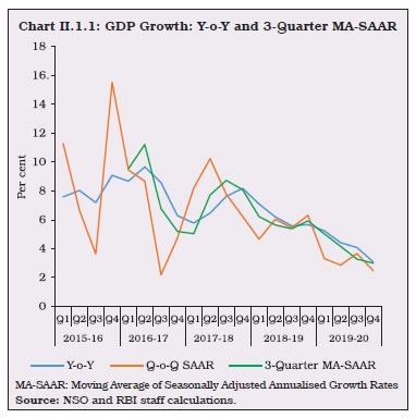
| Table II.1.1: Underlying Drivers of Growth | | Components | Growth (per cent) | Contribution to Growth (per cent) | | 2008-09 | 2009-11 | 2011-14 | 2014-18 | 2018-20 | 2008-09 | 2009-11 | 2011-14 | 2014-18 | 2018-20 | | 1 | 2 | 3 | 4 | 5 | 6 | 7 | 8 | 9 | 10 | 11 | | I. Total Consumption Expenditure | 5.5 | 6.5 | 6.1 | 7.5 | 7.0 | 118.2 | 53.5 | 71.5 | 64.6 | 91.8 | | Private | 4.5 | 5.9 | 6.7 | 7.4 | 6.2 | 81.9 | 40.4 | 66.2 | 53.8 | 68.5 | | Government | 11.4 | 9.7 | 2.6 | 8.2 | 10.9 | 36.3 | 13.1 | 5.3 | 10.8 | 23.3 | | II. Gross Capital Formation | -2.6 | 14.5 | 2.0 | 6.5 | 3.7 | -31.3 | 64.1 | 16.6 | 30.1 | 17.9 | | Fixed investment | 3.2 | 9.4 | 6.2 | 6.2 | 3.5 | 32.6 | 35.9 | 37.9 | 25.0 | 13.9 | | Change in stocks | -51.4 | 56.2 | -27.4 | 31.5 | 12.2 | -75.4 | 17.9 | -16.7 | 3.5 | 3.4 | | Valuables | 26.9 | 45.0 | -11.1 | 8.5 | 0.8 | 11.4 | 10.3 | -4.6 | 1.6 | 0.5 | | III. Net exports | | | | | | -72.4 | -4.1 | 8.9 | -8.5 | 14.0 | | Exports | 14.8 | 7.3 | 10.0 | 1.4 | 4.4 | 99.0 | 16.2 | 42.3 | 3.7 | 10.9 | | Imports | 22.4 | 6.9 | 6.1 | 4.2 | 0.9 | 171.4 | 20.3 | 33.4 | 12.3 | -3.0 | | IV. GDP | 3.1 | 8.2 | 5.7 | 7.7 | 5.2 | 100.0 | 100.0 | 100.0 | 100.0 | 100.0 | | Source: NSO and RBI staff calculations. | II.1.6 Compositional shifts in demand conditions reflect the anatomy of the persistent slowdown extending into 2019-20 (Chart II.1.2 and Appendix Table 2). Consumption II.1.7 Private final consumption expenditure (PFCE), constituting 57.2 per cent of aggregate demand, recorded its lowest growth in a decade. Nonetheless, at 5.3 per cent in 2019-20, PFCE growth exhibited resilience in the face of the prolonged weakening of income and financial conditions. High frequency indicators of consumption demand either contracted or grew at a rate far below their long-run averages. Petroleum consumption remained flat, while non-oil non-gold imports remained in contraction all through the year. Among indicators of urban demand, passenger car sales contracted throughout 2019-20, exacerbated by idiosyncratic factors such as rising insurance costs and tighter emission norms. Other indicators of urban demand, viz., consumer durables and air passenger traffic also remained depressed during the year, with the latter bearing the brunt of an exogenous shock due to the grounding of a major airline. 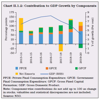 II.1.8 Among indicators of rural demand, tractor sales had contracted until the beginning of the rabi sowing season, but record sowing along with improvement in terms of trade for the farm sector revived demand and catalysed a spurt in tractor sales between December 2019 and February 2020 and stayed robust even during the pandemic period. Motorcycle sales, however, have remained in the contraction zone starting from January 2019. The weakness in rural demand was also aggravated by moderation in rural wages and dwindling employment avenues, and the slowdown in alternative sources of livelihood such as manufacturing and construction. GFCE compensated for the slowdown in private consumption, registering double-digit growth for the third consecutive year in 2019-20. Excluding GFCE growth of 11.8 per cent, GDP growth for 2019-20 would have decelerated by 0.9 percentage points from the headline GDP growth estimated by the NSO. The COVID-19 pandemic delivered an unprecedented shock to the economy. It remains to be seen whether the recovery from the pandemic will be V-shaped or U-shaped (Box II.1.1). Investment and Saving II.1.9 The rate of gross domestic investment in the Indian economy, measured by the ratio of gross capital formation (GCF) to GDP at current prices, had declined to 32.2 per cent in 2018-19. Although data on GCF are not yet available for 2019-20, underlying indicators point to investment having weakened further. The ratio of real gross fixed capital formation (GFCF) to GDP declined to 29.8 per cent in 2019-20 from 31.9 per cent in 2018-19 on account of waning business confidence. The corporate tax regime reform of September 2019 has not yet gained traction in boosting capital expenditure. Box II.1.1
Macroeconomic Impact of COVID-19 COVID-19’s epidemiological dynamics are still rapidly evolving in India, rendering difficult an accurate assessment of its full macroeconomic effects. In this scenario, an approach employing a dynamic stochastic general equilibrium (DSGE) model built on New Keynesian foundations provides a tentative and proximate assessment of the likely impact of COVID-19 and the subsequent lockdown on the Indian economy. The model has three main economic agents, viz., households, firms and the government. COVID-19 and the lockdown can impact the economy through multiple channels (Eichenbaum et al., 2020; Faria-e-Castro, 2020; Yang et al., 2020). Because of lockdown, households have to stay at home and therefore, reduce labour supply to firms; consumption falls due to non-availability of non-essential items and fall in income; and restricted people-to-people contact stalls the momentum of the pandemic. The model is calibrated2 so that infections peak around the second half of August 2020 [based on the predictions of a generalised Susceptible-Exposed-Infectious-Recovered (SEIR) model for India] and the output gap widens to about (-) 12 per cent of potential output when the economy is worst hit. Two scenarios are envisaged: the first, i.e., lockdown I, impacts the supply side of the economy by decreasing the labour supply and its productivity. The second scenario, i.e., lockdown II, additionally considers the increase in marginal cost. Inflation falls under both scenarios mainly because of a fall in demand; under lockdown II, however, the decline in inflation is less steep and short-lived. Firms respond to the squeeze in profits, due to higher marginal costs, by curtailing production and labour demand. Wages see a lower rise and economy goes through a large contraction. However, the recovery from the pandemic is faster in this scenario on account of fewer opportunities for people-to-people interactions. Under scenario I by contrast, production retrenchment is less severe, but demand contraction is more pronounced due to a rise in infections. Thus, the economy undergoes a deeper contraction under lockdown II, but recovery from the pandemic is faster (Chart 1). In order to evaluate the macroeconomic implications of scenarios I and II, it is worthwhile to simulate a third scenario in which the government does not impose a lockdown (Chart 2). This results in a more widespread pandemic, which peaks in the second half of January 2021 with a very slow recovery. This causes a persistent labour shortage and the supply shock produces a lasting impact on inflation and the output gap, which corresponds to a permanent upward shift in inflation and a downward shift in potential output, respectively. In scenario II, which envisages a second lockdown, the decline in economic activity is expected to reach its trough in Q1:2020-21 and growth turns positive from Q4:2020-213 (Chart 3a). Inflation, which was high at 6.7 per cent in Q4:2019-20, is projected to ease till Q4:2020-21 (Chart 3b). In sum, COVID-19 without the associated lockdown acts like a supply shock which causes a persistent rise in inflation and a permanent loss of output. As per Scenario II, which looks closer to the reality, the decline in economic activity reaches its trough in Q1:2020-21 and recovers thereafter, albeit at a gradual pace, with growth turning positive from Q4:2020-21. References: 1. Eichenbaum, M. S., S. Rebelo, and M. Traband (2020), ‘The Macroeconomics of Epidemics’, National Bureau of Economic Research, Working Paper No. 26882. 2. Faria-e-Castro, M. (2020), ‘Fiscal Policy during a Pandemic’, Federal Reserve Bank of St. Louis, Working Paper Series No. 06. 3. Yang, Y., H. Zhang, and X. Chen (2020), ‘Coronavirus Pandemic and Tourism: Dynamic Stochastic General Equilibrium Modeling of Infectious Disease Outbreak’, Annals of Tourism Research. | II.1.10 Another constituent of GFCF, viz., construction activity remained subdued in 2019-20 as a large inventory overhang coupled with stressed liquidity conditions restrained new launches. This was also reflected in growth of steel consumption, which plunged to a decadal low of 0.9 per cent in 2019-20 and cement production which registered a contraction of 0.9 per cent (Chart II.1.3). Driving the contraction in GFCF during 2019-20 was the collapse in investment in machinery and equipment, as evident in both imports and production of capital goods. II.1.11 As per the Order Books, Inventories and Capacity Utilisation Survey (OBICUS) of the Reserve Bank, capacity utilisation (CU) in manufacturing sector picked up from 68.6 per cent in Q3:2019-20 to 69.9 per cent in Q4:2019-20. On a seasonally adjusted basis, CU remained stable at 68.3 per cent in Q4:2019-20 as against 68.4 per cent in Q3:2019-20. II.1.12 The rate of gross domestic saving, measured as a ratio of gross domestic saving to gross national disposable income (GNDI), which had moderated to 29.7 per cent in 2018-19, is expected to gather pace during 2019-20 on the back of an uptick in household financial savings (Appendix Table 3). As per the preliminary estimates, household financial saving has improved to 7.6 per cent of GNDI in 2019-20, after touching the 2011-12 series low of 6.4 per cent in 2018-19 (Table II.1.2). This improvement has occurred on account of sharper moderation in household financial liabilities than that in financial assets. COVID-19 related economic disruptions, however, caused a sharper decline in household financial assets in Q4:2019-20. 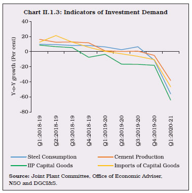
| Table II.1.2: Financial Saving of the Household Sector | | (Per cent of GNDI) | | Item | 2011-12 | 2012-13 | 2013-14 | 2014-15 | 2015-16 | 2016-17 | 2017-18 | 2018-19 | 2019-20# | | 1 | 2 | 3 | 4 | 5 | 6 | 7 | 8 | 9 | 10 | | A. Gross financial saving | 10.4 | 10.5 | 10.4 | 9.9 | 10.7 | 10.4 | 11.9 | 10.4 | 10.5 | | of which: | | | | | | | | | | | 1. Currency | 1.2 | 1.1 | 0.9 | 1.0 | 1.4 | -2.1 | 2.8 | 1.5 | 1.4 | | 2. Deposits | 6.0 | 6.0 | 5.8 | 4.8 | 4.6 | 6.3 | 3.1 | 4.1 | 3.6 | | 3. Shares and Debentures | 0.2 | 0.2 | 0.2 | 0.2 | 0.2 | 1.1 | 1.0 | 0.4 | 0.4 | | 4. Claims on Government | -0.2 | -0.1 | 0.2 | 0.0 | 0.5 | 0.7 | 0.9 | 1.0 | 0.0 | | 5. Insurance Funds | 2.2 | 1.8 | 1.8 | 2.4 | 1.9 | 2.3 | 2.0 | 1.3 | 1.7 | | 6. Provident and Pension funds | 1.1 | 1.5 | 1.5 | 1.5 | 2.1 | 2.1 | 2.1 | 2.1 | 2.1 | | B. Financial Liabilities | 3.2 | 3.2 | 3.1 | 3.0 | 2.7 | 3.0 | 4.3 | 4.0 | 2.9 | | C. Net Financial Saving (A-B) | 7.2 | 7.2 | 7.2 | 6.9 | 7.9 | 7.3 | 7.6 | 6.4 | 7.6 | GNDI: Gross National Disposable Income.
#: As per the preliminary estimate of the Reserve Bank. The NSO will release the financial saving of the household sector on January 29, 2021 based on the latest information, as part of the ‘First Revised Estimate of National Income, Consumption Expenditure, Saving and Capital Formation for 2019-20’.
Note: Figures may not add up to total due to rounding off.
Source: NSO. | 3. Aggregate Supply II.1.13 Aggregate supply, measured by gross value added (GVA) at basic prices, slowed to 3.9 per cent in 2019-20, 2.1 percentage points lower than a year ago and 2.8 percentage points below its decennial rate of 6.7 per cent. GVA’s momentum measured by three quarter moving average (MA) of quarter-on-quarter (q-o-q) seasonally adjusted annualised growth rates (SAAR) appears to have troughed in Q3:2019-20 and a modest uptick seems to have commenced in Q4:2019-20 (Chart II.1.4). II.1.14 On the supply side, the main locomotive of growth – the services sector – has been severely affected by the lockdown, while industrial GVA went into an accentuated contraction in 2019-20 (Table II.1.3). These negative tendencies were cushioned by the agriculture sector, as discussed below. 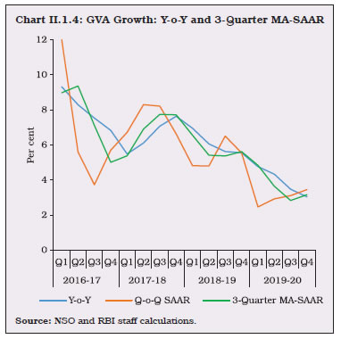
| Table II.1.3: Real GVA Growth | | Sectors | Growth (per cent) | Contribution to Growth (per cent) | | 2008-09 | 2009-11 | 2011-14 | 2014-18 | 2018-20 | 2008-09 | 2009-11 | 2011-14 | 2014-18 | 2018-20 | | 1 | 2 | 3 | 4 | 5 | 6 | 7 | 8 | 9 | 10 | 11 | | I. Agriculture, Forestry and Fishing | -0.2 | 4.0 | 4.5 | 3.3 | 3.2 | -1.2 | 8.7 | 14.6 | 6.9 | 10.6 | | II. Industry | 3.4 | 9.1 | 2.9 | 8.8 | 2.6 | 18.6 | 29.2 | 11.8 | 26.8 | 11.1 | | 2. Mining and Quarrying | -2.5 | 9.7 | -5.6 | 8.7 | -1.4 | -2.4 | 5.0 | -4.4 | 3.4 | -0.4 | | 3. Manufacturing | 4.7 | 9.3 | 4.5 | 8.9 | 2.9 | 18.5 | 22.2 | 14.1 | 20.9 | 8.7 | | 4. Electricity, Gas, Water Supply and Other Utility Services | 4.9 | 6.5 | 5.1 | 8.3 | 6.2 | 2.5 | 2.0 | 2.1 | 2.5 | 2.8 | | III. Services | 6.4 | 8.0 | 7.0 | 8.1 | 6.3 | 82.6 | 62.1 | 73.6 | 66.3 | 78.3 | | 5. Construction | 5.6 | 6.4 | 5.4 | 4.7 | 3.7 | 11.6 | 7.9 | 9.0 | 5.3 | 5.3 | | 6. Trade, Hotels, Transport, Communication and Services related to Broadcasting | 2.4 | 9.0 | 7.5 | 8.7 | 5.7 | 9.6 | 19.8 | 24.0 | 22.0 | 21.3 | | 7. Financial, Real Estate and Professional Services | 5.2 | 5.6 | 8.5 | 8.7 | 5.7 | 23.5 | 15.0 | 28.8 | 24.9 | 25.1 | | 8. Public Administration, Defence and Other Services | 15.8 | 11.8 | 5.1 | 8.4 | 9.7 | 37.8 | 19.4 | 11.7 | 14.1 | 26.6 | | IV. GVA at basic prices | 4.3 | 7.4 | 5.6 | 7.4 | 5.0 | 100.0 | 100.0 | 100.0 | 100.0 | 100.0 | | Source: NSO and RBI staff calculations. | II.1.15 Agriculture and allied activities, with a real GVA growth of 4.0 per cent in 2019-20 (PE), benefitted from record production of foodgrains as well as commercial and horticultural crops. The contribution of agriculture to overall economic growth (15.2 per cent) surpassed that of the industrial sector (4.7 per cent) for the first time since 2013-14. Although agriculture accounts for only 14.6 per cent share in overall GVA, the increased contribution in overall growth is expected to have positive impact on 48.3 per cent of total households who are employed in agriculture. II.1.16 The SWM started off on a sluggish note on June 8, 2019 with a delay of about one week from its normal onset. After a rainfall deficit of 33 per cent in June, the SWM gathered momentum from mid-July and cumulative rainfall at the end of the season (September 30, 2019) turned out to be 10 per cent above the long period average (LPA) [9 per cent below LPA during previous year]. Kharif sowing also gained momentum and ended the season with marginally higher acreage than in the previous year. Accordingly, kharif foodgrains production in 2019-20 is placed 1.3 per cent higher than the final estimates (FE) for 2018-19 (Table II.1.4). II.1.17 The incidence of cyclonic storms (mainly Vayu and Bulbul) and spells of unseasonal rains in October and mid-November (Chart II.1.5) resulted in damage to standing crops in many states. The maximum loss was in respect of urad, and production estimates were revised downward by 29.2 per cent (2nd AE over 1st AE) due to crop losses. | Table II.1.4: Agricultural Production 2019-20 | | (Lakh Tonnes) | | Crop | Season | 2018-19 | 2019-20 | 2019-20 Variation (Per cent) | | 4th AE | Final | Target | 4th AE | Over 2018-19 | Over 2019-20 | | 4th AE | Final | Target | | 1 | 2 | 3 | 4 | 5 | 6 | 7 | 8 | 9 | | Foodgrains | Kharif | 1,417.1 | 1415.2 | 1,479.0 | 1,433.8 | 1.2 | 1.3 | -3.1 | | | Rabi | 1,432.4 | 1437.0 | 1,432.0 | 1,532.7 | 7.0 | 6.7 | 7.0 | | | Total | 2,849.5 | 2852.1 | 2,911.0 | 2,966.5 | 4.1 | 4.0 | 1.9 | | Rice | Kharif | 1,021.3 | 1020.4 | 1,020.0 | 1,019.8 | -0.1 | -0.1 | 0.0 | | | Rabi | 142.9 | 144.4 | 140.0 | 164.5 | 15.1 | 13.9 | 17.5 | | | Total | 1,164.2 | 1164.8 | 1,160.0 | 1,184.3 | 1.7 | 1.7 | 2.1 | | Wheat | Rabi | 1,021.9 | 1036.0 | 1,005.0 | 1,075.9 | 5.3 | 3.9 | 7.1 | | Coarse Cereals | Kharif | 309.9 | 313.8 | 358.0 | 336.9 | 8.7 | 7.4 | -5.9 | | | Rabi | 119.6 | 116.7 | 125.0 | 137.9 | 15.3 | 18.2 | 10.3 | | | Total | 429.5 | 430.6 | 483.0 | 474.8 | 10.5 | 10.3 | -1.7 | | Pulses | Kharif | 85.9 | 80.9 | 101.0 | 77.2 | -10.1 | -4.6 | -23.6 | | | Rabi | 148.0 | 139.8 | 162.0 | 154.4 | 4.3 | 10.4 | -4.7 | | | Total | 234.0 | 220.8 | 263.0 | 231.5 | -1.1 | 4.8 | -12.0 | | Oilseeds | Kharif | 212.8 | 206.8 | 258.0 | 223.2 | 4.9 | 7.9 | -13.5 | | | Rabi | 109.8 | 108.5 | 103.0 | 111.1 | 1.2 | 2.4 | 7.8 | | | Total | 322.6 | 315.2 | 361.0 | 334.2 | 3.6 | 6.0 | -7.4 | | Sugarcane | Total | 4,001.6 | 4,054.2 | 3,855.0 | 3,557.0 | -11.1 | -12.3 | -7.7 | | Cotton # | Total | 287.1 | 280.4 | 358.0 | 354.9 | 23.6 | 26.6 | -0.8 | | Jute & Mesta ## | Total | 97.7 | 98.2 | 112.0 | 99.1 | 1.5 | 0.9 | -11.5 | #: Lakh bales of 170 kg each. ##: Lakh bales of 180 kg each. AE: Advance Estimate.
Source: Ministry of Agriculture and Farmers Welfare, GoI. |
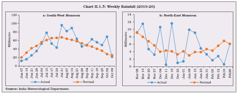 II.1.18 Overall foodgrains production is estimated at 2,966.5 lakh tonnes in 2019-20 – a record for the third successive year. Foodgrains production is estimated to have grown by 4.0 per cent in 2019-20, driven mainly by record production of rice and wheat. Among commercial crops, oilseeds, cotton, and jute and mesta are estimated to have grown by 6.0 per cent, 26.6 per cent and 0.9 per cent, respectively, while sugarcane production contracted by 12.3 per cent over the previous year. II.1.19 As per the 2nd AE, the production of horticultural crops reached a record level of 3,204.8 lakh tonnes during 2019-20, driven mainly by production of vegetables and fruits (Table II.1.5). All the three key vegetables – onions, tomatoes and potatoes – registered increased production. | Table II.1.5: Horticulture Production | | (Lakh Tonnes) | | Crops | 2017-18 | 2018-19 | 2019-20 | Variation (Per cent) | | Final Estimate (FE) | 2nd AE | Final Estimate (FE) | 2nd AE | 2018-19 FE over 2017-18 FE | 2019-20 2nd AE over 2018-19 2nd AE | 2019-20 2nd AE over the 2018-19 FE | | 1 | 2 | 3 | 4 | 5 | 6 | 7 | 8 | | Total Fruits | 973.6 | 973.8 | 979.7 | 990.7 | 0.6 | 1.7 | 1.1 | | Banana | 308.1 | 312.2 | 304.6 | 315.0 | -1.1 | 0.9 | 3.4 | | Citrus | 125.5 | 131.5 | 134.0 | 139.7 | 6.8 | 6.2 | 4.3 | | Mango | 218.2 | 209.6 | 213.8 | 204.4 | -2.0 | -2.5 | -4.4 | | Total Vegetables | 1,844.0 | 1,873.7 | 1,831.7 | 1,917.7 | -0.7 | 2.3 | 4.7 | | Onion | 232.6 | 232.8 | 228.2 | 267.4 | -1.9 | 14.8 | 17.2 | | Potato | 513.1 | 529.6 | 501.9 | 513.0 | -2.2 | -3.1 | 2.2 | | Tomato | 197.6 | 196.6 | 190.1 | 205.7 | -3.8 | 4.6 | 8.2 | | Plantation Crops | 180.8 | 176.6 | 163.5 | 162.4 | -9.6 | -8.0 | -0.7 | | Total Spices | 81.2 | 86.1 | 94.3 | 94.2 | 16.1 | 9.4 | -0.1 | | Aromatics and Medicinal | 8.7 | 8.5 | 8.0 | 8.0 | 3.9 | -6.6 | -0.4 | | Total Flowers | 27.9 | 28.9 | 29.1 | 30.6 | 4.1 | 5.8 | 5.5 | | Total | 3,117.4 | 3,148.7 | 3,107.4 | 3,204.8 | -0.3 | 1.8 | 3.1 | FE: Final Estimate. AE: Advance Estimate.
Source: Ministry of Agriculture and Farmers Welfare, GoI. | II.1.20 In recent years, the impact of climate change in terms of volatile rainfall intensity, increase in extreme events and rising temperature has implications for the outlook of agriculture (Box II.1.2). II.1.21 As in the previous two years, minimum support prices (MSPs) announced in 2019-20 for both rabi and kharif crops ensured a minimum return of 50 per cent over the cost of production. II.1.22 In the Union Budget 2020-21, the government had proposed to operationalise Kisan Rail for transporting perishable goods (including milk, meat and fish) to improve the efficiency of agricultural supply chains, reduce post-harvest losses and moderate price fluctuations. Further, Krishi Udaan scheme was proposed to help farmers to transport their produce by air on both national and international routes. The Budget has also given a major thrust to development of warehousing infrastructure as well as village level storage facilities in the country by involving various stakeholders such as NABARD, Warehouse Development and Regulatory Authority (WDRA), FCI, Central Warehousing Corporation (CWC) and self-help groups (SHGs). Pradhan Mantri Kisan Urja Suraksha evam Utthan Mahabhiyan scheme was launched enabling the farmers to set up solar power generation capacity on their fallow/ barren lands and to sell it to the grid. The government has proposed cluster-based 'One Product One District ' approach to tap the potential of horticulture sector in enhancing farmers’ income. Minimum support prices announced for kharif 2020-21 are higher by 2.9 per cent to 12.7 per cent vis-à-vis last year, ensuring a minimum return of 50 per cent over all India weighted average cost of production. Box II.1.2
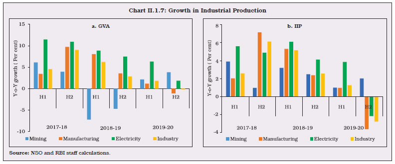
Climate Change - The Challenges for Indian Agriculture As in many parts of the world, drastic changes in climatic conditions have also been observed in India and these include impact on onset and withdrawal dates of monsoon and the incidence of extreme events (IPCC, 2019 and GoI, 2020). Consistent with models of climate change, the number of dry days as well as days with extremely high levels of rainfall have increased in India - more intense droughts; downward shifts in average rainfall by 59 mm since 2000 (Chart 1a); higher frequency of cyclones - India was hit by 8 cyclones in 2019 which is the highest since 1976 (Chart 1b); high variation in the number of subdivisions receiving excess/normal and deficient/scanty monsoon rains (Chart 1c); and an increase in the extent of crop area damaged due to unseasonal rains and heavy floods (Chart 1d). Global warming has also led to a sharp rise in the annual average temperature in India by 1.8°C between 1997 and 2019 as compared to a 0.5°C increase between 1901 and 2000 (Chart 2a). This has likely caused a decline in crop yields, undermining farm income (Chart 2b). Global warming has also led to a sharp rise in the annual average temperature in India by 1.8°C between 1997 and 2019 as compared to a 0.5°C increase between 1901 and 2000 (Chart 2a). This has likely caused a decline in crop yields, undermining farm income (Chart 2b). Water tables have depleted at an alarming rate, with around 52 per cent of the wells in India recording decline in water levels between the years 2008 and 2018 (Chart 3a). This imparts urgency to move from flood irrigation to micro irrigation methods like drip or hose reel, which can save up to 60 per cent of the water used and also help in preventing pest incidence. At present, the coverage of micro irrigation is much lower in states which have recorded higher declines in water tables (Chart 3b). Alongside, there is a need to adopt crop cycles, credit cycles and procurement patterns to monsoonal shifts. References: 1. Government of India, (2020), ‘Observed Monsoon Rainfall Variability and Changes during Recent 30 years (1989-2018)’, Climate Research and Services Division, Ministry of Earth Sciences, India Meteorological Department. 2. Intergovernmental Panel on Climate Change (IPCC) (2019), ‘Climate Change and Land’, World Meterological Organisation and United Nations Environment Programme. | II.1.23 Under Atmanirbhar Bharat Abhiyan Package, government has announced measures to strengthen infrastructure, logistics, capacity building, governance and administrative reforms for agriculture, animal husbandry, fisheries and food processing. These measures include eight development schemes4 with fund allocation of ₹1.6 lakh crore which is much higher as compared to funds allocated to the relevant schemes for the Union Budget 2020-21. In addition to the above schemes, the government has also announced three governance and administrative reforms to attract investments in agriculture sector and make it competitive, namely, delisting of various agricultural commodities from the Essential Commodities Act to develop seamless marketing and promote storage infrastructure in agriculture; ‘The Farmers’ Produce Trade and Commerce (Promotion and Facilitation) Ordinance 2020’ to ensure barrier free trade of agriculture produce; and ‘The Farmers (Empowerment and Protection) Agreement on Price Assurance and Farm Services Ordinance 2020’ to empower the farmers to engage with processors, aggregators, wholesalers, large retailers, and exporters in a fair and transparent manner (Annex II). Industrial Sector II.1.24 Industrial GVA decelerated sharply in 2019-20 to 0.8 per cent from 4.5 per cent last year. The print for 2019-20 was the lowest in the 2011-12 series, marking the fourth consecutive year of deceleration since 2015-16. The cyclical component5 of industrial GVA growth moved deeper into contraction (Chart II.1.6). II.1.25 The deceleration was broad-based with headwinds from subdued demand – both domestic and international. With dwindling confidence and imposition of lockdown, the demand for non-essential items plummeted. The index of industrial production (IIP) shrank by 0.8 per cent during 2019-20 from 3.8 per cent growth a year ago (Chart II.1.7a & 7b). II.1.26 In the manufacturing sector, which constitutes three-fourths of industry, 17 of 23 industry groups recorded contraction. The motor vehicles segment was the largest negative contributor to manufacturing IIP, while basic metals, largely comprising mild steel slabs, provided a positive impetus. II.1.27 The mining sector decelerated largely on account of disruptions caused by extended monsoon. Crude oil and natural gas production declined due to depletion in reserves, flood repairs and industrial strikes, in addition to sluggish demand. There was some recovery in mining activity during H2 as unfavourable weather conditions waned and economic activity picked up in January-February 2020. Electricity generation decelerated due to contraction in thermal power generation, lean industrial demand and the extended monsoon. IIP manufacturing and electricity closely co-moved, indicating that a pick-up in manufacturing activities is essential for electricity demand to improve. Hydro electricity generation registered double digit growth during the year even as the share of renewables increased in the total electricity generation mix. 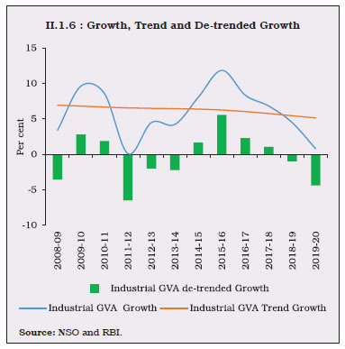
 II.1.28 In terms of use-based classification, much of the deceleration in IIP was caused by a sharp contraction in capital goods and consumer durables production (Table II.1.6). | Table II.1.6: Index of Industrial Production (2011-12 = 100) | | (Per cent) | | Industry Group | Weight in IIP | Growth Rate | | 2015-16 | 2016-17 | 2017-18 | 2018-19 | 2019-20 | 2019-20
(April-June) | 2020-21
(April-June) | | 1 | 2 | 3 | 4 | 5 | 6 | 7 | 8 | 9 | | Overall IIP | 100 | 3.3 | 4.6 | 4.4 | 3.8 | -0.8 | 3.0 | -35.9 | | Mining | 14.4 | 4.3 | 5.3 | 2.3 | 2.9 | 1.6 | 3.0 | -22.4 | | Manufacturing | 77.6 | 2.8 | 4.4 | 4.6 | 3.9 | -1.4 | 2.4 | -40.7 | | Electricity | 8.0 | 5.7 | 5.8 | 5.4 | 5.2 | 1.0 | 7.3 | -15.8 | | Use-Based | | | | | | | | | | Primary goods | 34.0 | 5.0 | 4.9 | 3.7 | 3.5 | 0.7 | 2.6 | -20.3 | | Capital goods | 8.2 | 3.0 | 3.2 | 4.0 | 2.7 | -13.9 | -3.5 | -64.4 | | Intermediate goods | 17.2 | 1.5 | 3.3 | 2.3 | 0.9 | 9.1 | 9.2 | -43.0 | | Infrastructure/ construction goods | 12.3 | 2.8 | 3.9 | 5.6 | 7.3 | -3.6 | 0.4 | -48.3 | | Consumer durables | 12.8 | 3.4 | 2.9 | 0.8 | 5.5 | -8.7 | -2.7 | -67.6 | | Consumer non-durables | 15.3 | 2.6 | 7.9 | 10.6 | 4.0 | -0.1 | 7.0 | -15.3 | | Source: NSO. | II.1.29 In terms of weighted contributions to IIP, the shares of capital goods, construction/ infrastructure goods, consumer durables and consumer non-durables declined, while that of intermediate goods increased (Chart II.1.8). II.1.30 Even as the persisting weakness in capital goods production, and the decline in capacity utilisation have raised concerns in the context of investment slowdown, demand for consumer non-durables has also slumped, suggesting overall weakening of demand conditions (Chart II.1.9). II.1.31 The deceleration in manufacturing activity is aggravated by decline in trade due to trade disruptions with the onset of COVID-19 and declining demand. The import intensity of India’s manufacturing products6, on an average, stood at 35.6 per cent during the period 2015-17 (Table II.1.7).
II.1.32 Import intensity differs across product groups, with the electronics industry having the highest import dependence, followed by machinery and equipment, reflecting disproportionate impact of trade restrictions on industries. Accordingly, an import disruption, ceteris paribus, would lead to non-availability of crucial components, resulting in contraction in manufacturing GVA by as much as 2.5 per cent (Table II.1.8). | Table II.1.7: Select Industry-wise Import Dependence (Average of 2015-2017) | | (Per cent) | | Industry | Import Intensity of Intermediate Inputs | Import Intensity of Output | Share in Manufacturing GVA | | 1 | 2 | 3 | 4 | | Electronics | 60.7 | 42.8 | 4.6 | | Machinery | 48.5 | 37.3 | 8.1 | | Transport Equipment | 5.3 | 3.4 | 11.5 | | Chemicals | 29.4 | 21.0 | 9.0 | | Pharmaceuticals | 2.7 | 1.3 | 6.5 | | Total Manufacturing | 35.6 | 25.1 | 100.0 | | Source: RBI staff estimates. | II.1.33 The impact due to factor income loss (capital and labour) of 68 days of lockdown on the manufacturing and mining sectors could be as high as ₹2.7 lakh crore (Table II.1.9). Services Sector II.1.34 In tandem with the slowdown in the industrial sector, services sector growth decelerated to 5.0 per cent in 2019-20 – the lowest in the last three decades. All sub-sectors except public administration, defence and other services (PADO) decelerated, the latter cushioning overall services sector growth, despite revenue shortfalls. Excluding PADO, services sector GVA growth decelerated to 3.7 per cent from 7.0 per cent in 2018-19 (Chart II.1.10). | Table II.1.8: Impact of Trade Disruption in India’s Manufacturing Sector | | (Per cent) | | India’s Main Imports | Global Import | | Scenario I: Import Freezes | Scenario II: Import < 50 per cent | Scenario III: Import < 25 per cent | | 1 | 2 | 3 | 4 | | Capital Goods (Machinery) | 0.84 | 0.42 | 0.21 | | Electronics and Electricals | 0.83 | 0.41 | 0.21 | | Pharmaceuticals | 0.05 | 0.01 | 0.01 | | Chemicals | 0.70 | 0.18 | 0.18 | | Transport Equipment | 0.16 | 0.02 | 0.04 | | Combined Effect on GVA of the Above Sectors | 2.58 | 1.04 | 0.64 | | Total Manufacturing GVA | 9.90 | 4.95 | 2.48 | Note: All values should be read as negative.
Source: RBI staff estimates |
| Table II.1.9: Impact on Manufacturing and Mining GVA - Alternate Scenarios | | Sectors | Disruptions | Factor Income Loss Estimated in Constant Prices (₹ lakh crore) | | Phase I & II: Lockdown (40 days) | Phase III & IV: Lockdown (28 days) | Cumulative Effect (68 days) | | 1 | 2 | 3 | 4 | 5 | | Mining & Quarrying | Partial | 0.389 | 0.109 | 0.498 | | Manufacturing | Partial | 1.664 | 0.576 | 2.240 | | Manufacturing & Mining GVA | | 2.053 | 0.685 | 2.738 | Note: 1. The sectoral proportion of labour income shares are taken from India KLEMS database.
2. All values to be read as negative.
3. The Q1:2020-21 impact on manufacturing GVA considers 33 days in Phase I & II, 28 days in Phase III & IV and 61 days in cumulative effect.
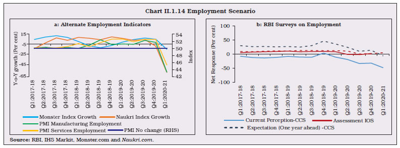
Source: RBI staff estimates. | II.1.35 Deceleration in construction and trade, hotels, transport, communication and services related to broadcasting drove the slowdown in overall services activity (Chart II.1.11). II.1.36 The sluggishness in the road transport sector was reflected in a contraction in commercial vehicle sales that began since H2:2018-19 and intensified through the year. The air transport segment remained stagnant, with contraction in both passenger and cargo traffic. Foreign tourist arrivals fell sharply from February 2020 pointing to difficult times ahead for the hospitality industry in the wake of COVID-19. The hospitality industry is likely to be the worst affected sector globally. Even rail transport decelerated during 2019-20. The construction sector registered its sharpest deceleration – from 6.1 per cent in 2018-19 to 1.3 per cent during 2019-20. Private sector estimates indicates that in the housing sector, new launches and sales declined in Q4:2019-20. II.1.37 The Reserve Bank’s services sector composite index (SSCI)7, which tracks activity in construction, trade, transport and finance and is a coincident indicator of GVA growth in the services excluding PADO, declined in 2019-20 (Chart II.1.12). 4. Employment II.1.38 In June 2020, the NSO released the Periodic Labour Force Survey (PLFS) of employment for 2018-19. The labour force participation rate was estimated at 37.5 per cent in 2018-19, an increase of 0.6 percentage points from 2017-18. The unemployment rate according to usual status declined to 5.8 per cent in 2018-19 (6.0 per cent for male and 5.2 per cent for female) from 6.1 per cent in 2017-18 (6.2 per cent for male and 5.7 per cent for female). Worker population rate, an indicator of employment, increased to 35.3 per cent in 2018-19 as compared to 34.7 per cent in 2017-18. In terms of distribution of workers by broad status in employment, the share of regular wage/salaried workers increased from 22.8 per cent in 2017-18 to 23.8 per cent in 2018-19, with a corresponding fall in the proportion of casual workers from 24.9 per cent to 24.1 per cent during the same period, indicating enhanced formalisation of the economy. 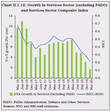 II.1.39 More updated organised sector employment, measured in terms of payroll8 data from the Employees’ Provident Fund Organisation (EPFO), Employees’ State Insurance Corporation (ESIC) and National Pension System (NPS), indicated a mixed picture with regard to job creation in 2019-20 (Chart II.1.13). Net subscribers added to EPFO per month averaged 6.5 lakh during April-March 2019-20, up from 5.6 lakh a year ago. On the other hand, the average number of members who paid their contribution to ESIC contracted by 4.1 lakh during 2019-20, in contrast to an addition of 0.6 lakh during 2018-19. New subscribers to NPS increased marginally during the same period. II.1.40 For Q4:2019-20, PMI employment index showed payroll hiring in manufacturing gained momentum whereas, for services, the rate of job creation moderated as compared to previous quarter. Hiring activity measured by online recruitment, showed a mixed pattern. While Naukri Job Speak Index contracted sharply, Monster Employment Index registered growth during Q4:2019-20 (Chart II.1.14a). Both the Industrial Outlook Survey (IOS) and Consumer Confidence Survey (CCS) pointed to the sentiments on employment conditions remaining pessimistic during Q4:2019-20 (Chart II.1.14b). 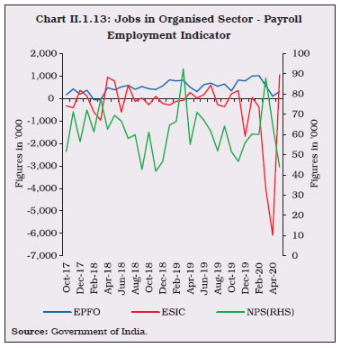
 II.1.41 Considering the small farm size in India, the self-employed in agriculture can be assumed to be relatively unscathed by the pandemic. On the other hand, 40 per cent of casual labourers in rural areas are employed in the construction sector, which has come to a complete halt during the lockdown (Table II.1.10). Self-employed and casual labourers together account for 51.3 per cent of the urban workforce, and hence, the pandemic has disproportionate impact on urban areas. II.1.42 Several policy initiatives were undertaken by the government during the year for addressing structural bottlenecks in the economy. These policies are aimed at generating employment opportunities such as strategic promotion of labour-intensive manufacturing, increasing public expenditure on MGNREGA, Prime Minister’s Employment Generation Programme (PMEGP), Pandit Deen Dayal Upadhyaya Grameen Kaushalya Yojana (DDU-GKY) and Deen Dayal Antodaya Yojana – National Urban Livelihoods Mission (DAY-NULM). For skill development, a target to train over 69.03 lakh during 2016-17 to 2019-20 has been set to help them earn a livelihood through Pradhan Mantri Kaushal Vikas Yojana. As a part of legislative reforms, 44 labour laws have been simplified, amalgamated and rationalised into 4 labour codes in accordance with the recommendations of the 2nd National Commission on Labour. The Code on Wages, 2019, passed in both the Houses of Parliament, is expected to bring greater formalisation of the labour market and safeguard interests of workers, while facilitating employment creation and ease of doing business. | Table: II.1.10: Sector and Area-wise Type of Workforce | | (Percentage Share in respective Employment Category) | | Sectors | Rural | Urban | Rural+ Urban | | Self employed | Regular /Salaried | Casual | Self employed | Regular/ Salaried | Casual | Self employed | Regular/ Salaried | Casual | | 1 | 2 | 3 | 4 | 5 | 6 | 7 | 8 | 9 | 10 | | Agriculture | 73.9 | 4.7 | 49.9 | 10.5 | 0.5 | 9.3 | 60.4 | 2.1 | 43.6 | | Mining & Quarrying | 0.1 | 1.1 | 0.8 | 0.1 | 0.8 | 0.4 | 0.1 | 0.9 | 0.6 | | Manufacturing | 6.5 | 20.0 | 4.7 | 22.8 | 23.6 | 17.1 | 10.0 | 22.2 | 6.7 | | Electricity & Water Supply | 0.1 | 1.8 | 0.1 | 0.7 | 1.7 | 0.2 | 0.2 | 1.9 | 0.1 | | Construction | 1.9 | 3.2 | 40.0 | 4.7 | 2.5 | 51.7 | 2.5 | 2.8 | 42.0 | | Trade, Hotel & Restaurant | 10.9 | 13.3 | 1.0 | 34.6 | 17.9 | 7.6 | 16.0 | 16.1 | 1.7 | | Transport, Storage & Communication | 3.0 | 12.7 | 2.3 | 12.3 | 9.8 | 8.1 | 4.9 | 10.7 | 3.3 | | Other Services | 3.5 | 43.3 | 1.2 | 14.3 | 43.2 | 5.6 | 5.8 | 43.3 | 1.9 | | Total | 100.0 | 100.0 | 100.0 | 100.0 | 100.0 | 100.0 | 100.0 | 100.0 | 100.0 | | Source: RBI staff calculations. | II.I.43 A package of measures was announced in May 2020 under Atmanirbhar Bharat Abhiyan in five tranches cover, among others, rural employment generation, infrastructure, MSMEs, NBFCs, migrant workers and ease of doing business. These measures aggregate around ₹20 lakh crore or 10 per cent of GDP and aim to address the difficulties faced by various categories including MSMEs, NBFCs, power distribution companies and infrastructure projects. The measures, both short-term and long-term in nature, also endeavour to make India self-reliant by boosting private participation in numerous sectors with global quality and competitiveness. The growth of India’s personal protective equipment (PPE) sector from scratch before March 2020 to making 1,50,000 pieces a day by beginning of May 2020 shows the potential of India in meeting the challenges. II.I.44 MSMEs which are badly hit by the pandemic are expected to benefit from various policies of the government such as collateral free loan of ₹3 lakh crore, subordinate debt provision of ₹20,000 crore and equity infusion via mother-fund-daughter fund model. Further, the change in definition of classification of MSMEs by including turnover as basis of definition will allow MSMEs to expand without losing benefits and also improve ease of doing business by aligning them with GST. The structural reforms introduced as part of fourth tranche of stimulus is expected to bring in private investments across eight critical sectors9. The proposed change in public sector enterprise policy, where all sectors will be opened to private sectors, and public-sector enterprises will operate only in notified strategic sectors, will bring in far-reaching changes in India’s industrial sector. The Atmanirbhar Bharat Abhiyan Package aims to provide immediate relief to sections of the economy most impacted by the pandemic and to revive economic activity along with creating new opportunities for employment and growth. In the manufacturing sector, 100 per cent FDI in contract manufacturing and commercial coal mining through the automatic route is expected to bring in more private investments. II.1.45 To sum up, consumption demand slumped during 2019-20. Gross fixed capital formation could not sustain its past momentum and contracted. On the supply side, agriculture and allied activities accelerated with record foodgrains and horticulture production supported by allied activities, which remained robust. Industrial sector activity plummeted during 2019-20, driven down mostly by the manufacturing sub-sector. With services sector growth also decelerating, the outlook for the economy is clouded by uncertainty and testing challenges, mainly the intensity, spread and duration of COVID-19. The priority is to revive growth as the Indian economy heals from the scars of COVID-19. II.2 PRICE SITUATION II.2.1 The global inflation environment remained benign through 2019 and the early part of 2020, engendered by soft commodity prices and massive monetary policy accommodation. In India too, headline inflation10 was benign in the first half of 2019-20, but firmed up in the second half due to a sharp spike in food inflation on a combination of adverse developments, i.e., the late withdrawal of the monsoon, unseasonal rains and supply disruptions. During December 2019-February 2020, headline inflation breached the upper tolerance band for inflation mandated for the monetary policy committee (MPC) [Chart II.2.1]. II.2.2 In the event, annual average inflation crossed 4 per cent for the first time since the adoption of flexible inflation targeting (FIT) framework in 2016, amidst accentuated volatility (Table II.2.1). The intra-year distribution of inflation also had a high positive skew, reflecting the spikes in food inflation during the second half of the year. Furthermore, kurtosis turned slightly less negative than it was a year ago, suggesting a few instances of large deviations from mean inflation, which was also reflected in the wide gap between maximum and minimum inflation during the year. 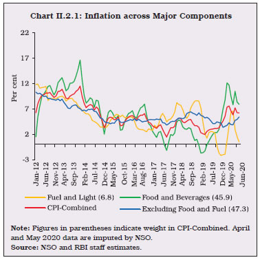
| Table II.2.1: Headline Inflation – Key Summary Statistics | | (Per cent) | | | 2012-13 | 2013-14 | 2014-15 | 2015-16 | 2016-17 | 2017-18 | 2018-19 | 2019-20 | | 1 | 2 | 3 | 4 | 5 | 6 | 7 | 8 | 9 | | Mean | 10.0 | 9.4 | 5.8 | 4.9 | 4.5 | 3.6 | 3.4 | 4.8 | | Standard Deviation | 0.5 | 1.3 | 1.5 | 0.7 | 1.0 | 1.2 | 1.1 | 1.8 | | Skewness | 0.2 | -0.2 | -0.1 | -0.9 | 0.2 | -0.2 | 0.1 | 0.5 | | Kurtosis | -0.2 | -0.5 | -1.0 | -0.1 | -1.6 | -1.0 | -1.5 | -1.4 | | Median | 10.1 | 9.5 | 5.5 | 5.0 | 4.3 | 3.4 | 3.5 | 4.3 | | Maximum | 10.9 | 11.5 | 7.9 | 5.7 | 6.1 | 5.2 | 4.9 | 7.6 | | Minimum | 9.3 | 7.3 | 3.3 | 3.7 | 3.2 | 1.5 | 2.0 | 3.0 | Note: Skewness and Kurtosis are unit-free.
Source: NSO and RBI staff estimates. | II.2.3 Against this backdrop, sub-section 2 assesses developments in global commodity prices and inflation. Sub-section 3 discusses movements in headline inflation and major turning points, followed by a detailed analysis of the major constituents of inflation in sub-section 4. Sub-section 5 discusses other indicators of prices and costs, followed by concluding observations. 2. Global Inflation Developments II.2.4 International food prices were range-bound during H1:2019-20, but they firmed up from October 2019, primarily led by wheat (due to strong international demand), maize (supply uncertainty in the US and Argentina), palm oil (lower supply and rising demand for biodiesel in producing countries), meat (demand from China) and fish prices (Chart II.2.2). Beginning December 2019, prices of rice (drought conditions in Thailand), sugar (lower than expected world production) and other edible oils also hardened. In the non-food category, metal prices remained weak due to US-China trade tensions and subdued global demand. Prices of precious metals, however, registered a sharp increase on safe haven demand amidst global uncertainties. Crude oil prices generally declined during May-August 2019, despite production cuts by the organisation of the petroleum exporting countries (OPEC) and ongoing geopolitical tensions. A supply disruption in Saudi Arabia in September 2019 caused prices to increase temporarily before falling in October 2019. Prices picked up during November-December 2019 on hopes of positive US-China trade talks and deepening of production cuts by OPEC+ from 1.2 million barrels per day (mbpd) to 1.7 mbpd. In January 2020, however, the COVID-19 pandemic hit the transportation sector, which accounts for more than 60 per cent of oil demand. This led to a fall in crude oil prices during January-February 2020 to a level of US$ 5311 per barrel in February 2020. Subsequently, crude oil prices plunged even lower to US$ 32.2 per barrel in March 2020 as the OPEC+ failed to reach an agreement on production cuts. The price of the Indian basket of crude oil touched US$ 33.4 per barrel in March 2020, the lowest since February 2016. As the COVID-19 pandemic spread across the globe, all commodity prices dipped. The shutdown of industries in China in February 2020 and later in Europe and the US led to a fall in demand for metals, easing their prices. Prices of food items like palm oil, soy oil, sugar and corn also declined with retrenchment in demand for ethanol and bio-diesel as crude oil prices declined. Prices of some food items like rice and wheat were, however, supported by stockpiling by consumers in regions affected by COVID-19. Despite OPEC+ reaching an agreement to cut oil production by about 10 mbpd (about 10 per cent of global supply) in early April, crude oil prices continued to fall on COVID-19 induced slump in demand and exhaustion of storage capacity. Brent crude oil prices fell to a low of US$ 23.3 per barrel in April 2020. Subsequently, crude prices did recover to around US$ 42.8 per barrel in July 2020, but remained far below pre-COVID-19 levels. 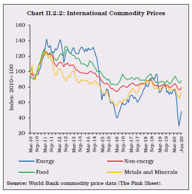 II.2.5 Reflecting these global commodity price developments and weak demand conditions, consumer price inflation remained benign during 2019 and early 2020 in a number of economies. Core consumer price inflation was low in advanced economies (AEs), despite robust job growth. Many emerging market and developing economies (EMDEs) also experienced easing of inflation due to subdued economic activity, although some pressures from rising food prices were visible. With the outbreak of COVID-19 and consequential lockdown bringing global economic activity to near standstill, many economies resorted to monetary and fiscal measures to ward off recessionary tendencies and provide support to growth. 3. Inflation in India II.2.6 After trending below the target of 4 per cent during the first half of 2019-20, headline inflation spiked during the second half and reached a multi-year peak of 7.6 per cent in January 2020 (highest in 68 months) [Chart II.2.3]. An atypically prolonged south west monsoon (SWM) along with unseasonal rains during the kharif harvest period led to crop damages and supply disruptions which pushed up food prices, especially those of vegetables, from September to December 2019. Thereafter, with the fading of these pressures and encouraging prospects for the rabi crop, food inflation started easing from January 2020. II.2.7 Fuel prices recorded five consecutive months of deflation during July-November 2019, before bouncing back during December 2019-March 2020 on the pressures from international prices of LPG and kerosene. Inflation excluding food and fuel remained generally moderate during the year, with a historic low in October 2019, before gradually picking up again till January 2020. II.2.8 For the year as a whole, inflation picked up to average 4.8 per cent in 2019-20, 136 basis points (bps) higher than a year ago (Appendix Table 4). With the uptick in headline inflation from September 2019, households’ median inflation expectations hardened during the second half of 2019-20 by 103 bps three months ahead and by 133 bps a year ahead. This upturn in expectations is also corroborated by more forward-looking assessments of professional forecasters and by surveys of consumer confidence. 4. Constituents of CPI Inflation II.2.9 Constituents of CPI headline inflation exhibited distinct shifts during 2019-20 (Chart II.2.4). During the first half of the year, food inflation trailed below headline inflation, whereas inflation excluding food and fuel ruled above it. The dynamics reversed during the second half, with food inflation remaining significantly above the headline and inflation excluding food and fuel pacing below it. Inflation in fuel prices had eased below headline inflation from February 2019 to February 2020, but rose above it in March 2020. Food II.2.10 Inflation in prices of food and beverages (weight: 45.9 per cent in CPI) leaped from 1.4 per cent in April 2019 to 12.2 per cent in December 2019. Consequently, its contribution to overall inflation surged to 57.8 per cent in 2019-20 from 9.6 per cent a year ago. The delay in the onset of the southwest monsoon (SWM) by around a week, followed by a considerably longer delay in withdrawal (by 39 days), led to the persistence of high momentum in food prices. Additionally, cyclonic storms and unseasonal rains resulted in supply disruptions and damage to kharif crops, primarily vegetables and pulses, during December-January 2019-20 (Chart II.2.5). Price pressures soon became broad-based and were also observed across items such as cereals, milk, eggs, meat and fish, and spices. The delayed winter easing of vegetables prices brought some relief during January-March 2020. II.2.11 Drilling down into specific pressure points, prices of vegetables (weight: 13 per cent in CPI-Food and beverages) shaped the overall food inflation trajectory during 2019-20. Excluding vegetables, food inflation would have averaged 236 bps lower in 2019-20 (6.0 per cent including vegetables). The crop damage, mentioned earlier, resulted in a historically high build-up of momentum; consequently, vegetables price inflation rose to an all-time high of 60.5 per cent in December 2019 (Chart II.2.6a). II.2.12 Within vegetables, onion prices dominated the build-up in upside pressures (Chart II.2.6b) right from June 2019 in the wake of a slump in mandi arrivals due to reduced rabi onion acreage in Maharashtra in drought-like conditions. In addition, unseasonal rains during September-October 2019 damaged the kharif onion crop in major producing states of Maharashtra, Madhya Pradesh, Karnataka and Andhra Pradesh, escalating prices from September 2019. 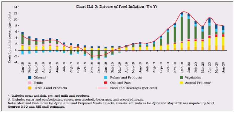
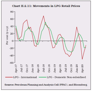
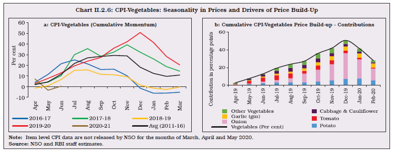 Furthermore, the rains also impacted the transplantation of the late kharif onion crop. Onion price inflation skyrocketed to 327.4 per cent in December 2019. Supply side measures, including imposing a minimum export price (MEP) of US$ 850 per tonne, banning export of onions, imposing stock holding limits on wholesale traders and retailers in September 2019, and announcement of import of 1.2 lakh tonnes of onions from Turkey, Afghanistan and Egypt during November-December 2019 did not, however, fully alleviate price pressures. With the arrival of the delayed kharif crop and on the back of a better rabi crop, which boosted the production of onions, as per the 2nd Advance Estimates (AE) of the Ministry of Agriculture, onion prices started easing from January 2020. II.2.13 Potato prices also picked up throughout the year (barring September 2019 and February 2020), primarily due to untimely and excess rains, which damaged crops ready for harvest and disrupted supplies to mandis. Consequently, potato price inflation reached an all-time high of 63 per cent in January 2020, after emerging out of 7 months of continuous deflation in November 2019. In the case of tomato prices, inflation peaked at 70 per cent in May 2019 and remained in high double digits till December 2019, due to delayed harvesting in Maharashtra and fungus-damaged crops in Karnataka, coupled with the supply disruptions referred to earlier in key supplier states – Karnataka, Maharashtra and Himachal Pradesh. Tomato prices, however, moderated during November 2019 - February 2020, in line with the usual seasonal pattern. II.2.14 Prices of cereals and products (weight of 21 per cent in the CPI-Food and beverages) also witnessed a build-up in upside pressures during 2019-20 (Chart II.2.7), rising almost continuously from 1.2 per cent in April 2019 to around 5.3 per cent during January-March 2020. In the case of wheat, inflation averaged around 6.5 per cent during the year, capped by higher procurement which also economised on imports (31.4 per cent lower in 2019-20). Non-PDS rice prices emerged out of 11 months of deflation in October 2019 on account of positive price pressures and unfavourable base effects to reach an inflation level of 4.2 per cent in January 2020, in the wake of higher procurement and damages to the kharif crop, but they moderated to 3.9 per cent in February 2020.  II.2.15 Milk and products prices (weight of 14.4 per cent in the CPI-Food and beverages) were another pressure point during the year (Chart II.2.8). Increase in procurement prices of milk led to major milk co-operatives like Amul and Mother Dairy raising retail milk prices by ₹2-3 per litre twice – during May and again in December 2019. This was followed by similar hikes by milk co-operatives in other states, elevating the momentum of milk and products prices during the year. Increases in the cost of production because of reduced availability of fodder also contributed to an upward revision in procurement prices and, subsequently, in retail prices. Higher global prices for skimmed milk products also supported milk prices. Milk price inflation peaked during the year at 6.5 per cent in March 2020. 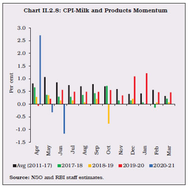 II.2.16 In the case of pulses (weight: 5.2 per cent in CPI-Food and beverages), 2019-20 began with the end of a prolonged deflation of 29 months in May 2019. Ahead of this development, a substantial fall (by 54 per cent) in imports during 2018-19 had helped in rebalancing the demand-supply situation. Additionally, a decline in kharif pulses production (by 4.6 per cent as per 4th Advance Estimates for 2019-20 over 2018-19 Final Estimates), especially urad production (by 44.9 per cent), added to inflation persistence (Chart II.2.9), despite imports being higher by around 14.6 per cent during 2019-20. II.2.17 Inflation in protein-rich items such as eggs and meat and fish (weight: 8.8 per cent in CPI-Food and beverages) averaged 4.5 per cent and 9.3 per cent, respectively – the highest in the last six years – and together, they contributed 13.7 per cent of overall food inflation during the year. Meat and fish prices reflected higher feed prices, especially of maize and soybean. Along similar lines, egg prices witnessed heightened prices during September-January 2019-20. With the outbreak and spread of COVID-19, however, the consumption of poultry slumped and prices moderated during February-March 2020. II.2.18 Among other major food items, sugar and confectionery, and oils and fats also contributed positively to overall food inflation, reflecting a decline in domestic production in the case of the former and higher international prices in respect of the latter. II.2.19 Prices of fruits (weight of 6.3 per cent in the CPI-food and beverages group) emerged out of nine months of deflation in September 2019 but prices generally remained soft in the rest of the year. Prices of spices, especially of dry chillies and turmeric, registered significant pressures due to a reduction in the area under production. Fuel II.2.20 The contribution of the fuel group (weight of 6.8 per cent in CPI) to headline inflation decreased to 1.9 per cent in 2019-20 from 11.3 per cent in the previous year. Fuel inflation eased sequentially from April to June 2019 and moved into deflation during July-November 2019, pulled down by favourable base effects and muted price pressures in major fuel items (Chart II.2.10). Domestic LPG prices, which rose during April-June 2019, sank into deflation in July 2019, tracking the collapse in international LPG prices with a lag (Chart II.2.11). Firewood and chips inflation picked up during December 2019 to February 2020 on the back of strong price pressures on winter demand. Domestic LPG prices also moved out of deflation in January 2020, in line with the upward movement in international LPG prices. Administered kerosene prices continued to rise throughout 2019-20 as oil marketing companies (OMCs) raised prices in a calibrated manner to eventually phase out the kerosene subsidy. Electricity inflation, which had largely remained in negative territory during April-August 2019, also recorded an uptick in H2:2019-20. Reflecting these developments and strong unfavourable base effects, fuel inflation turned positive in December 2019 and reached an intra-year peak of 6.6 per cent in March 2020. 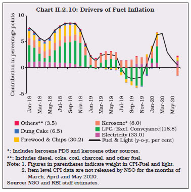
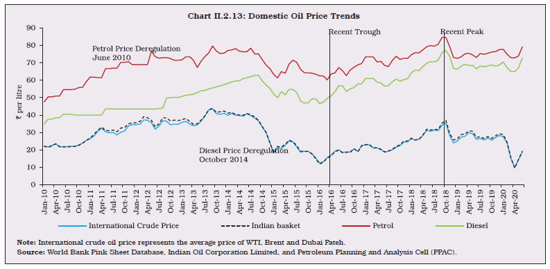
 Inflation Excluding Food and Fuel II.2.21 Inflation excluding food and fuel moderated from 2018-19 levels to an average of 4.0 per cent in 2019-20 (Appendix Table 4) with a historic low of 3.4 per cent in October 2019 (Chart II.2.12). Some hardening occurred during November 2019-January 2020 due to prices of personal care and effects and transport and communication sub-groups, reflecting increase in gold prices, hikes in mobile telecom tariffs, and the rise in petrol and diesel prices (Chart II.2.13). Subsequently, a sharp fall in transport and communication prices in February and March 2020 on the back of easing international crude oil prices and falling domestic air passenger traffic led to moderation during February-March 2020. II.2.22 Among the major constituents of this group, inflation in prices of the miscellaneous category moderated during April-October 2019 reaching 3.4 per cent in October 2019 (lowest since July 2017) and again during February-March 2020. Within the miscellaneous group, price pressures remained generally contained in respect of household goods and services, health, recreation and amusement, and education. II.2.23 Housing inflation moderated to 4.5 per cent in 2019-20 (6.7 per cent in 2018-19), reflecting the waning of the impact of the increase in house rent allowance (HRA) for central government employees under the 7th Pay Commission award. A historic low of 3.7 per cent was recorded in March 2020. Net of housing, inflation excluding food and fuel averaged 3.9 per cent in 2019-20, down from 5.6 per cent a year ago. II.2.24 Clothing and footwear inflation eased to a trough of 1.0 per cent in September 2019, largely reflecting muted input costs. International prices of cotton, a major input into clothing production, as measured by the Cotton A Index, fell during May to August 2019, followed by a recovery during September 2019-January 2020. The outbreak of COVID-19 also rattled international cotton markets, with the Cotton A Index registering a fall in February and March 2020. 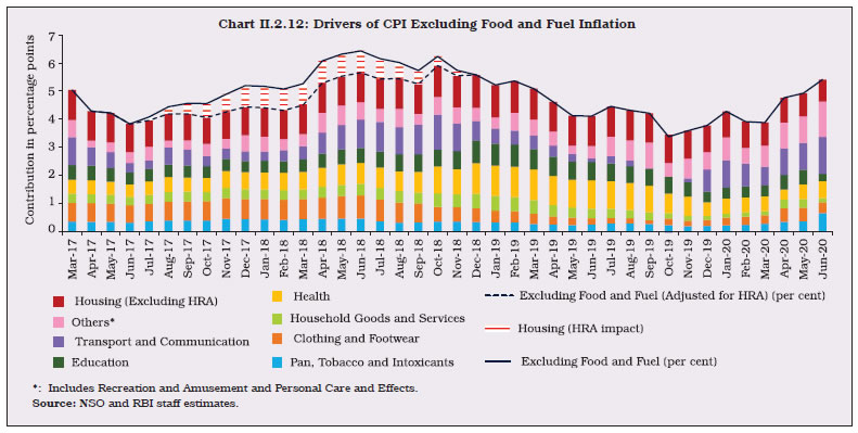
 II.2.25 Overall, headline inflation was subjected to higher volatility in 2019-20 relative to the previous four years, underpinned by high flux in food prices (Charts II.2.14a & b). Within the food group, price spikes for different items occurred at different time points. Empirical analysis for the period January 2011 and February 2020 suggests that seasonal behaviour has changed in the case of prices of many food items such as, onions, ginger, brinjals, cauliflowers, okras and green peas. Interestingly, despite being the most volatile item, seasonality in onion prices has declined significantly over the years, partly reflecting improvement in cold storage facilities. Volatility estimated from asymmetric GARCH12 models suggest volatility in onion prices is likely to persist in the near term, while tomato price volatility may be short-lived. Inflation is persistent in the case of protein items and dry fruits, more than that for prices of vegetables. There is no evidence of persistence of volatility in prices of items such as petrol, diesel and precious metals, although these items also contribute to volatility in headline inflation. 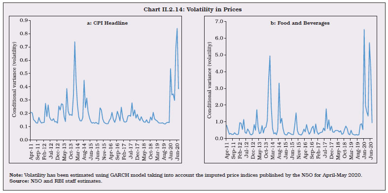 5. Other Indicators of Inflation II.2.26 During 2019-20, sectoral CPI inflation based on the consumer price index of industrial workers (CPI-IW) remained elevated and reached 9.6 per cent in December 2019 (highest in 73 months), primarily due to housing and food prices. With the impact of HRA revision of the 7th central pay commission (CPC) completely waning in January 2020 and food prices easing along with favourable base effects, CPI-IW inflation softened to 5.5 per cent in March 2020. Inflation based on the consumer price index of agricultural labourers (CPI-AL) and the consumer price index of rural labourers (CPI-RL), which do not have housing components, also increased during the year and reached 11.1 per cent and 10.6 per cent, respectively, in December 2019 (highest in 72 months) before easing thereafter, on softening of food prices and favourable base effects. II.2.27 Inflation, measured by the wholesale price index (WPI), remained subdued during 2019-20. It reached an intra-year low of zero per cent in October 2019 (lowest in 40 months) due to deflation in prices of non-food manufactured products and fuel and power. It picked up during November 2019-January 2020, however, driven by a sharp uptick in prices of primary articles and unfavourable base effects, before moderating to 0.4 per cent in March 2020 due to softening in the prices of all three major groups, i.e., primary articles, fuel & power and manufactured products. On an annual average basis, WPI inflation softened to 1.7 per cent in 2019-20 from 4.3 per cent in 2018-19. A similar easing was also visible in the GDP deflator to 2.9 per cent in 2019-20 from 4.6 per cent in 2018-19. II.2.28 After major increases in minimum support prices (MSPs) during 2018-19 for kharif and rabi crops, MSPs witnessed a moderate hike in 2019-20. The extent of MSP increases varied across crops, ranging from 1.1 per cent in the case of moong and nigerseed to 9.1 per cent for yellow soybean. MSPs of rice and wheat were increased by 3.7 per cent and 4.6 per cent, respectively. II.2.29 Wage growth for agricultural and non-agricultural labourers generally remained subdued during the year, averaging around 3.4 per cent, and reflecting the slowdown in the construction sector. In the corporate sector, pressures from staff costs remained moderate during the year. II.2.30 In sum, headline inflation picked up strongly during the closing months of 2019-20 and the short-term outlook for food inflation has turned uncertain. Global crude oil prices have started firming modestly in more recent weeks. Disruptions in food and manufactured items’ supply chains could amplify sectoral price pressures, thus posing an upside risk to headline inflation. Heightened volatility in financial markets could also have a bearing on inflation. All of these may influence inflation expectations of households, which are adaptive in nature, and show significant sensitivity to shocks to food and fuel prices. Monetary policy, therefore, has to keep a constant vigil on price movements, especially as they can translate into generalised inflation. II.3 MONEY AND CREDIT II.3.1 Monetary and credit conditions moderated through 2019-20 reflecting the weakening of underlying economic activity, with inflation remaining benign in the first half of the year before spiking on food price pressures in the later months. The rate of money supply (M3) slackened as deposit growth moderated. Towards the close of the year, the slowing of deposit growth became accentuated as COVID-19 impelled a flight to cash. In terms of the sources of money supply, credit growth slumped to half its rate a year ago, reflecting weak demand and risk aversion among banks. Contra-cyclically, reserve money (RM) expansion, adjusted for first round effects of cash reserve ratio (CRR) changes, was broadly maintained at the preceding year’s rate, bolstered by a build-up of net foreign assets (NFA) of the Reserve Bank and its monetary policy operations in consonance with the accommodative policy stance adopted since June 2019 – open market purchases; reduction in the CRR; special market operations (in the form of long-term repo operations and targeted long-term repo operations); and USD/INR swaps. These developments engendered abundant liquidity in the system which eased liquidity premia in the midst of strong discrimination by financial markets on credit risk concerns. II.3.2 Against this backdrop, sub-section 2 delves into the dynamics underlying movements in RM and, thereby, into the role of the Reserve Bank’s balance sheet in the larger context of the state of the economy. This section also analyses the impact of COVID-19 on currency in circulation. Sub-section 3 examines developments in money supply in terms of its components and sources, throwing light on the behaviour of assets and liabilities of the banking sector. The underpinnings of bank credit evolution during the year have been covered in sub-section 4. This is followed by concluding observations and some policy perspectives. 2. Reserve Money II.3.3 Reserve money – a stylised depiction of the Reserve Bank’s balance sheet that focuses on its ‘moneyness’13 comprising currency in circulation, bankers’ deposits and other deposits with the Reserve Bank – increased by 9.4 per cent in 2019-20, lower than 14.5 per cent a year ago as well as its decennial trend rate of 11.4 per cent (2010-19) [Chart II.3.1; Appendix Table 4]. Adjusted for the reduction in the CRR by 100 basis points (bps), effective March 28, 2020 – which reduced RM statistically by around ₹1,37,000 crore – RM grew by 13.7 per cent during the year, as against 13.9 per cent in 2018-19. II.3.4 Drilling into the unravelling of reserve money changes during the year reveals interesting behavioural shifts. Among components, the expansion in RM was driven by currency in circulation (CiC) – 120 per cent of the RM expansion during the year. At the end of March 2020, CiC constituted around 81 per cent of RM. II.3.5 The demand for CiC normally follows a defined intra-month pattern – expansion during the first fortnight due to transactions by households, followed by a contraction in the second fortnight due to flow back of currency from households to the banking system (Chart II.3.2). II.3.6 CiC also exhibits seasonality across months/quarters – expanding in Q1, followed by contraction in Q2, with more than three-fourths of its annual variation occurring during Q3 and Q4. The year 2019-20 began with the usual seasonal spurt in currency demand in Q1 associated with summer holidays, weddings, rabi procurement and kharif sowing. In the following quarter, CiC contracted due to seasonal slack of economic activity in cash-intensive sectors such as construction and agriculture. Thereafter, CiC expanded, reflecting rise in currency demand for kharif harvest and festivals in Q3 and the harvest of rabi crops during Q4. The year ended with a surge in pandemic-related rush to cash. Overall, CiC growth of 14.5 per cent was slightly lower vis-a-vis 16.8 per cent a year ago (Chart II.3.3); however, the currency-GDP ratio increased to its pre-demonetisation level of 12.0 per cent in 2019-20 from 11.3 per cent a year ago, indicating the rise in cash-intensity in the economy in response to the pandemic (Chart II.3.4). 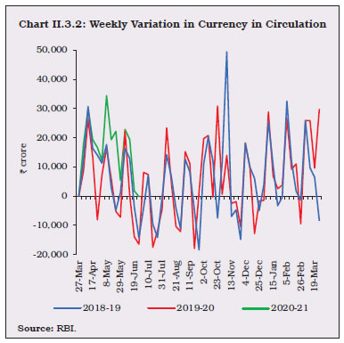 II.3.7 There was an unusual rise in month-over-month (M-o-M) CiC variation during March-June 2020 vis-à-vis the corresponding period in previous years14 (Chart II.3.5 and Chart II.3.6).
II.3.8 Bankers’ deposits with the Reserve Bank decreased by 9.6 per cent in 2019-20 as against an increase of 6.4 per cent in the previous year, mirroring subdued deposit mobilisation and the reduction in CRR to 3.0 per cent for a period of a year, effective March 28, 2020 (Chart II.3.7).
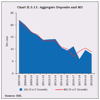
II.3.9 Amongst sources of RM, net domestic assets (NDA) and NFA have alternated in determining RM growth (Chart II.3.8). During 2019-20, the main driver was NFA, with net purchases from Authorised Dealers at ₹3,12,005 crore vis-à-vis net sales at ₹1,11,945 crore in the previous year. Consistent with the accommodative stance of monetary policy set out in June 2019, the Reserve Bank ensured comfortable liquidity conditions, augmenting its liquidity management toolkit with unconventional instruments. II.3.10 Net open market purchases of ₹1.1 lakh crore resulted in an increase in net Reserve Bank credit to the government by ₹1.9 lakh crore, which became the main driver of NDA in 2019-20. Among other constituents of NDA, net claims on banks15 and the commercial sector (mainly PDs), reflected mainly net LAF absorption aimed at sterilising forex operations and managing the large overhang of liquidity in the system (Chart II.3.9). II.3.11 The net LAF position was in repo mode during April-May 2019, but turned into reverse repo mode for the remainder of the financial year (Chart II.3.10a and Chart II.3.10b). 3. Money Supply II.3.12 M3, comprising currency with the public (CwP), aggregate deposits (AD) and other deposits with the Reserve Bank, averaged 10.2 per cent for the first three quarters of 2019-20 (10.1 per cent a year ago), before dropping off sharply in February and March 2020 to end the year at 8.9 per cent (Chart II.3.11). II.3.13 From the components side, M3 expansion was contributed by AD, its largest constituent (86 per cent), led mainly by time deposits – AD accounted for 78 per cent of the increase in M3 during the year. On a year-on-year basis, however, there was a moderation in time deposit growth due to the decline in interest rates and the general slowdown in economic activity (Chart II.3.12). As usual, demand deposits remained volatile, mirroring largely the variations in CwP (Chart II.3.13), which grew at a lower rate of 14.5 per cent vis-à-vis 16.6 per cent in the previous year. The flight towards cash and a concomitant drawdown on demand deposits was particularly visible in the last quarter of 2019-20, in the wake of uncertainities related to COVID-19 pandemic. 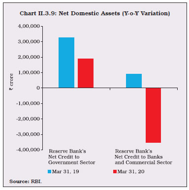
 II.3.14 Bank credit to the commercial sector, followed by net bank credit to the government and net foreign exchange assets of the banking sector, led the expansion in M3. Nonetheless, bank credit to the commercial sector grew at a lower rate than a year ago, reflecting lower bank credit offtake in the economy (Chart II.3.14 and Table II.3.1). With non-SLR investments of banks also decelerating, commercial banks augmented their SLR portfolios, which was reflected in net bank credit to government increasing by 11.8 per cent as compared with 9.7 per cent a year ago. Growth of NFA of the banking sector mirrored NFA in RM.
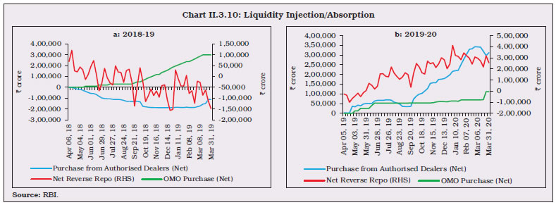
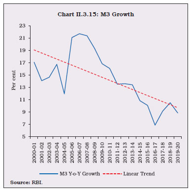
Key Monetary Ratios II.3.15 The money multiplier declined to 5.5 by end-March 2020 from 5.6 a year ago, converging towards its decennial average level (2010-19) of 5.5. Adjusted for reverse repo, however, analytically akin to banks’ deposits with the central bank – the money multiplier turned out to be lower at 4.8 by end-March 2020, reflecting the deceleration in the rate of money supply below its secular trend (Chart II.3.15). 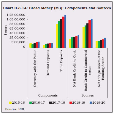
| Table II.3.1: Monetary Aggregates | | Item | Outstanding as on March 31, 2020
(₹ Crore) | Year-on-year growth rate
(in per cent) | | 2018-19 | 2019-20 | 2020-21
(as on June 19, 2020) | | 1 | 2 | 3 | 4 | 5 | | I. Reserve Money (RM) | 30,29,674 | 14.5 | 9.4 | 11.8 | | II. Money Supply (M3) | 167,99,930 | 10.5 | 8.9 | 12.3 | | III. Major Components of M3 | | | | | | III.1. Currency with the Public | 23,49,715 | 16.6 | 14.5 | 21.3 | | III.2. Aggregate Deposits | 144,11,708 | 9.6 | 8.0 | 10.9 | | IV. Major Sources of M3 | | | | | | IV.1. Net Bank Credit to Government | 49,06,583 | 9.7 | 11.8 | 19.8 | | IV.2. Bank credit to Commercial Sector | 110,38,644 | 12.7 | 6.3 | 6.3 | | IV.3. Net Foreign Assets of the Banking Sector | 38,01,036 | 5.1 | 23.8 | 27.4 | | V. M3 net of FCNR(B) | 166,18,480 | 10.5 | 8.8 | 12.5 | | VI. Money Multiplier | 5.5 | | | | Note: 1. Data are provisional.
2. The data for RM pertain to June 26, 2020.
Source: RBI. |
 II.3.16 Linking this phenomenon of money creation process to the dynamics of economic activity, empirical analysis16 considering data from Q1:2010 to Q4:2019 suggests that the money multiplier adjusted for reverse repo could be a lead indicator for gauging the movement of economic activity. Also, the money multiplier adjusted for reverse repo appears to be a better indicator, capturing the recent dynamics of economic activity more closely than the unadjusted money multiplier. II.3.17 The currency-deposit ratio at 16.3 per cent at end-March 2020 moved above its decennial average (2010-19) of 15.1 per cent. During the year, the pace of expansion in currency and a rise of the currency-deposit ratio pointed to a shift in public’s preference towards holding cash in response to the uncertainty caused by the pandemic. As at end-March 2020, the reserve-deposit ratio was 3.8 per cent (4.5 per cent last year), reflecting the impact of the CRR reduction (Chart II.3.16). II.3.18 With the statutory requirements for CRR and statutory liquidity ratio (SLR), at 3 per cent and 18 per cent, respectively, around 79 per cent of deposits were available with the banking system as on end-March 2020 for credit expansion. The moderation in the credit-deposit ratio to 76.4 per cent as at end-March 2020 from 77.7 per cent a year ago was largely a reflection of subdued demand conditions in the economy due to several factors examined subsequently. II.3.19 The credit-deposit ratio, which measures the demand for credit relative to funding available in the banking system, underwent four distinct phases since independence. It varied with the evolution of the economy – from the pre-nationalisation phase to the post-nationalisation phase, and subsequently, the reform phase starting from early 1990s followed by movements dictated by upturns and downturns in growth cycles. These movements also reflected changes in statutory requirements for CRR and SLR. The average credit-deposit ratio of 72 per cent during the first two post-independence decades fell to 69 per cent during the next two decades as deposit growth gained momentum with the geographic spread of banking services, and further to 55 per cent during 1990-2004 due to phases of subdued credit demand. Subsequently, the average credit-deposit ratio increased to 75 per cent during 2005-20 on the back of a credit boom (2005-14), and supportive economic growth conditions (Chart II.3.17). 4. Credit II.3.20 Credit offtake from SCBs was muted during 2019-20, growing at 6.1 per cent y-o-y in a sharp loss of pace from 13.3 per cent a year ago and from a recent peak of 15.0 per cent in December 2018. II.3.21 Credit demand has been ebbing away across all sectors, despite the post-IL&FS shift among large borrowers, including non-banking financial companies (NBFCs) and housing finance companies (HFCs), away from non-bank sources and towards the banking system for meeting funding requirements. The unabated weakening of economic activity, coupled with deleveraging of corporate balance sheets and risk aversion by banks due to asset quality concerns, was accentuated towards the close of the year by the pandemic woes (Chart II.3.18), producing a reduction in the incremental credit-deposit ratio (Chart II.3.19). The credit-to-GDP gap remained wide during 2019, reflecting the slack in credit demand (Chart II.3.20). II.3.22 The COVID-19 outbreak has affected more than 200 countries across the globe, bringing global economic activity to a near standstill, through lockdown and social distancing norms necessary for the safety and health concerns of the human beings. Several fiscal and monetary policy measures were also undertaken in India in sync with other countries to mitigate the macroeconomic impact caused by the pandemic (Annex II). With a nation-wide lockdown and people mostly remaining indoors, amidst fear and uncertainty, the usage of cash witnessed an abnormal rise (Chart II.3.21). The Reserve Bank undertook expansionary monetary policy measures to ensure the availability of adequate liquidity in the system. COVID-19 has imparted scars on monetary and credit aggregates towards the end of the year (Box II.3.1). 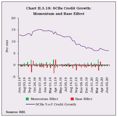
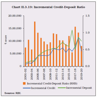
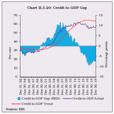 II.3.23 Data on sectoral deployment of bank credit17 for March 2020 point to a broad-based slowdown. Credit growth to agriculture and allied activities, and industry – mainly large and medium units – decelerated in 2019-20. However, credit growth to micro and small industries accelerated. Within industry, credit growth to beverage and tobacco, mining and quarrying, petroleum, coal products and nuclear fuels and rubber, plastic and their products accelerated whereas flows to chemicals and chemical products, cement and cement products and construction decelerated. Credit growth to food processing, basic metal and metal products and infrastructure contracted (Table II.3.2 & Chart II.3.22a). 
Box II.3.1
Impact of COVID-19 on Monetary and Credit Aggregates Many economies, especially in the emerging world, where the virus has spread rapidly, experienced the phenomenon of rising cash in circulation. Cross-country monetary statistics (IMF, 2020) indicate that the increase in currency in circulation was particularly sharp in Brazil, Chile, India, Russia and Turkey, as also in advanced economies such as the US, Spain, Italy, Germany and France, where the use of cash is less (Chart 1). The rise in currency in circulation in these countries occurred concomitantly with liquidity injecting measures undertaken by their central banks. They were also impacted by the COVID-19 build-up of precautionary balances. 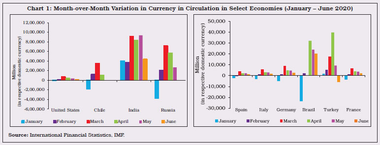 Concurrently, the World Uncertainty Index (WUI) and the World Pandemic Uncertainty Index (WPUI) of the economies mentioned above remained high during Q1:2020 (Chart 2 and 3). Rising uncertainty reduces the willingness of businesses to invest money and generate employment opportunities whereas, on the other hand, it reduces consumer spending (Ahir, et al. 2020). A spurt in the number of confirmed COVID-19 cases in India after March 13, 2020 accentuated the deceleration of deposit growth that had commenced from February 2020, essentially reflecting a ‘dash to cash’ under extreme uncertainty (Chart 4). Concomitantly, the y-o-y growth in currency with the public (CwP) accelerated from 11.3 per cent as on February 28, 2020 to 14.5 per cent at end-March 2020 and to 21.3 per cent by June 19. By contrast, bank credit, which had decelerated continuously during the year, has remained largely stable through the COVID-19 outbreak despite sharp contraction in activity levels. 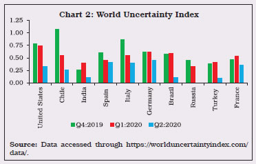
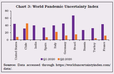
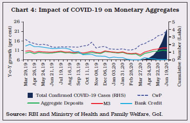 Reflecting these developments, the credit-deposit (C-D) ratio increased from 75.8 per cent at end-January 2020 to 76.4 per cent at end-March 2020, led by the increased demand for cash for transactions as digital payments declined. Post-March 2020, the easing was primarily due to a sharp rise in deposits, driven by a heightened propensity to save in response to the uncertainty caused by COVID-19 (Chart 5). Reference: Ahir, H., Bloom, N. and Furceri, D. (2020). ‘60 Years of Uncertainty’, Finance and Development, March. | II.3.24 Credit growth to infrastructure contracted during 2019-20, mainly due to reduction in offtake by the power segment and deceleration in credit flows to the roads and telecommunications segments. Credit to the services sector decelerated sharply, primarily driven down by slowdown in credit growth to NBFCs, on account of concerns relating to the health of the sector. There was also a sharp deceleration in credit to the trade segment. Personal loan growth decelerated moderately. Housing loans, which constitute the largest segment of personal loans, witnessed a moderate deceleration, along with credit cards outstanding. However, there was an acceleration in growth of vehicle loans during the year. II.3.25 As on March 27, 2020, non-food credit (NFC) growth decelerated to 6.7 per cent from 12.3 per cent last year. Among bank groups, credit growth by public sector banks (PSBs) decelerated sharply to 3.4 per cent in March 2020 from 10.2 per cent a year ago, reflecting stress from impaired balance sheets. Credit growth by private sector banks also decelerated to 13.9 per cent in March 2020 from 17.5 per cent a year ago, mainly attributable to deceleration in credit growth to the services sector (Chart II.3.22a and Chart II.3.22b). II.3.26 To sum up, even as monetary and credit conditions moderated through 2019-20, COVID-19 led to an unusual surge in currency demand, along with deceleration in aggregate deposits. Credit growth weakened during the year, with deceleration in all major sectors. The Reserve Bank pro-actively managed liquidity conditions through conventional and unconventional measures to augment system-level liquidity. Going forward, surplus liquidity conditions, coupled with policy rate reductions, are expected to instill confidence, easing financial conditions and incentivising the flow of funds at affordable rates so as to rekindle investment and lay the foundations of strong sustainable growth as the COVID-19 curve flattens and the economy repairs and revives. | Table II.3.2: Credit Deployment to Select Sectors | | Sectors | Outstanding as on March 27, 2020
(₹ Crore) | Year-on-Year Growth (Per cent) | | 2018-19* | 2019-20# | 2020-21## | | 1 | 2 | 3 | 4 | 5 | | Non-food Credit (1 to 4) | 92,11,544 | 12.3 | 6.7 | 6.7 (11.1) | | 1. Agriculture & Allied Activities | 11,57,795 | 7.9 | 4.2 | 2.4 (8.7) | | 2. Industry (Micro & Small, Medium and Large) | 29,05,151 | 6.9 | 0.7 | 2.2 (6.4) | | 2.1. Micro & Small | 3,81,825 | 0.7 | 1.7 | -3.7 (0.6) | | 2.2. Medium | 1,05,598 | 2.6 | -0.7 | -9.0 (2.2) | | 2.3. Large | 24,17,728 | 8.2 | 0.6 | 3.7 (7.6) | | (i) Infrastructure | 10,53,913 | 18.5 | -0.2 | 4.2 (15.2) | | of which: | | | | | | (a) Power | 5,59,774 | 9.5 | -1.6 | 0.9 (9.7) | | (b) Telecommunications | 1,43,760 | 36.7 | 24.4 | 36.8 (20.9) | | (c) Roads | 1,90,676 | 12.2 | 2.0 | 4.7 (14.6) | | (ii) Chemicals & Chemical Products | 2,02,949 | 17.5 | 6.0 | 3.1 (11.1) | | (iii) Basic Metal & Metal Product | 3,50,325 | -10.7 | -5.7 | -0.5 (-10.3) | | (iv) Food Processing | 1,54,146 | 1.1 | -1.9 | 4.2 (1.2) | | 3. Services | 25,94,945 | 17.8 | 7.4 | 10.7 (13.0) | | 4. Personal Loans | 25,53,652 | 16.4 | 15.0 | 10.5 (16.6) | | 5. Priority Sector | 28,97,461 | 7.3 | 5.8 | 1.9 (10.2) | *: March 2019 over March 2018. #: March 2020 over March 2019. ##: June 2020 over June 2019.
Note: 1. Data are provisional.
2. Figures in parentheses indicate growth rates in June 2019 over June 2018.
Source: RBI. |
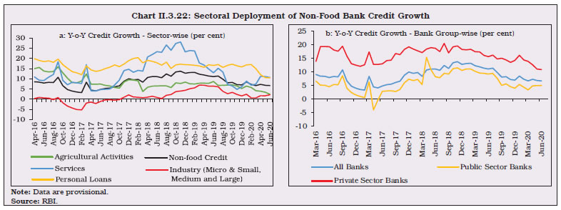
II.4 FINANCIAL MARKETS II.4.1 Global financial markets, which traded on a buoyant note during most part of 2019 and early 2020, experienced panic sell-offs across asset classes, triggered by the outbreak of COVID-19. Volatility soared to extraordinarily high levels, reminiscent of the turbulence seen during the global financial crisis (GFC). As investors scrambled into US dollar positions to seek safe haven, depreciations set in upon almost all other currencies. Bond yields firmed up on massive sell-offs, but speedy central bank actions with widespread policy rate cuts and large amounts of liquidity injection along with fiscal measures appeared to have calmed sentiment. II.4.2 In India, equity market also fell sharply in sync with global markets with the outbreak of COVID-19. After the announcement of the corporate tax rate cut in September 2019, it made handsome gains and rose to record new highs in January 2020 on the back of positive sentiments on US-China trade talks and the likelihood of an orderly Brexit. However, this positive momentum was interrupted by the escalation of geo-political tensions between the US and Iran, weakening domestic growth prospects and higher inflation expectations. COVID-19 brought an abrupt change in sentiments in March 2020. After exhibiting range-bound two-way movements with weakening bias during first three quarters, Indian rupee depreciated to an all-time low during Q4:2019-20 on large capital outflows from both the equity and debt markets. In the money market, as detailed in sub-section 2, overnight money market rates (call money, triparty repo, and market repo) were largely aligned with the policy rates albeit with a downward bias, and were insulated from adverse global developments by proactive liquidity management by the Reserve Bank. Bond yields softened significantly during 2019-20 as discussed in sub-section 3, aided initially during H1:2019-20 by positive sentiments from the general election results, policy rate cuts, infusion of liquidity by the Reserve Bank and the possibility of the fiscal deficit slippage being contained. During H2:2019-20, yields softened further on the back of auction of special OMOs, softening of US treasury yields, easing crude oil prices and announcement of comprehensive liquidity measures on March 27, 2020 to mitigate the adverse impact of COVID-19. Sub-section 4 profiles developments in the corporate bond market wherein yields softened during 2019-20, reflecting policy rate cuts by the MPC and injection of systemic liquidity, especially through the special OMOs and Long-term Repo Operations (LTRO) conducted during the latter part of the year. Sub-section 5 presents developments in the domestic equity market, followed by a discussion on movements in the Indian rupee in the foreign exchange market in sub-section 6. The section concludes with some forward-looking perspectives. 2. Money Market II.4.3 The money market remained generally stable during 2019-20, especially in H1. In the second half of the year, bouts of volatility, mainly in March 2020 on account of the spread of COVID-19, dispelled the calm. II.4.4 Beginning June 2019, liquidity conditions transited gradually out of deficit conditions during Q1:2019-20. The Reserve Bank proactively managed frictional liquidity conditions with a slew of conventional liquidity measures, viz., reduction in the CRR and easing of daily maintenance requirements, variable and fixed rate repos/ reverse repos of various tenors and access to the Marginal Standing Facility (MSF) as well as several unconventional measures, including long-term repo operations (LTRO), targeted long-term repo operations (TLTRO), line of credit to financial institutions, and a special liquidity facility for mutual funds (MFs). II.4.5 The weighted average call rate (WACR) in the unsecured inter-bank call money market remained aligned with the policy repo rate during the year with a downward bias (Chart II.4.1). The average absolute spread of the WACR over the policy rate increased to 11 basis points (bps) in 2019-20 from 9 bps in 2018-19, as surplus liquidity conditions prevailed in the banking system for most of the year. II.4.6 Volatility in the call money segment, measured by the coefficient of variation18 of the WACR, increased to 7.55 in 2019-20 from 3.40 a year ago, reflecting the swings in liquidity conditions. The triparty repo and market repo rates remained below the WACR, on average, by 22 bps each. 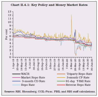 II.4.7 Average daily volume in the money market (call money, triparty repo and market repo taken together) increased by 16 per cent to ₹2,42,658 crore during 2019-20 from ₹2,09,152 crore in 2018-19. Volumes in the triparty repo and market repo segments increased by 24 per cent and 9 per cent, respectively. The share of triparty repo and market repo segments were 68 per cent and 25 per cent, respectively, of the total money market volume during 2019-20 as compared with 64 per cent and 27 per cent, respectively, in 2018-19. In the call money segment, average daily volumes decreased by 17 per cent during the year to ₹16,558 crore, reducing its market share to 7 per cent from 9 per cent in the previous year. The traded volumes in both secured and unsecured money market segments increased in recent months, in spite of COVID-19. II.4.8 Interest rates on longer tenor money market instruments, viz., 91-day Treasury Bills (T-bills), certificates of deposit (CDs) and commercial papers (CPs) generally moved in sync with the policy repo rate during 2019-20. The spread of CD rates over T-bill rates narrowed in Q3:2019-20 to 21 bps from 39 bps in Q2; however, it widened to 48 bps in Q4 following the outbreak of COVID-19 and the usual year-end balance sheet phenomenon (Chart II.4.2). II.4.9 In the primary market, fresh issuances of CDs decreased to ₹3.88 lakh crore during 2019-20 as compared with ₹5.65 lakh crore in the previous year. New issuances of CPs in the primary market declined to ₹21.95 lakh crore in 2019-20 from ₹25.96 lakh crore in 2018-19. The weighted average discount rates in the primary CP market hardened from September 2019 until mid-October 2019 on increased risk perceptions resulting from defaults and rating downgrades of a few NBFCs. However, it softened by 10 bps to 5.78 per cent by end-February 2020, as risks subsided, before hardening marginally to stand at 6.15 per cent at end-March 2020. 3. G-sec Market II.4.10 G-sec yields hardened in April 2019 in response to the Reserve Bank maintaining a neutral monetary policy stance contrary to market expectation, sustained higher crude oil prices following the US announcement of stopping of imports from Iran and supply disruptions in Libya and Venezuela, and depreciation of the Indian rupee (INR). In the rest of Q1:2019-20, the benchmark G-sec yield softened by 47 bps, taking positive cues from the general election results, infusion of liquidity by the Reserve Bank and lower crude oil prices. Market sentiment was buoyed further by the MPC’s decision to reduce the policy repo rate by 25 bps to 5.75 per cent on June 6, 2019 coupled with the change in policy stance from neutral to accommodative. The yield on the 10-year benchmark security softened from 7.35 per cent at end-March 2019 to 6.88 per cent on June 29, 2019 with some intermittent upswings. II.4.11 The softening of G-sec yields continued with a decline in yield by 20 bps in Q2:2019-20, barring some hardening in August and September 2019. Notwithstanding a larger than expected policy rate cut of 35 bps by the Reserve Bank, rollback of surcharge on foreign portfolio investments (FPIs) and higher than expected surplus transfer by the Reserve Bank, market participants remained wary in August and September with the yield hardening by 19 and 14 bps, respectively, on concerns over fiscal slippage and geo-political tensions following the attack on Saudi oil refineries. II.4.12 In Q3:2019-20, G-sec yields moved in a narrow range during October-November 2019, before hardening in the first fortnight of December 2019. Initially, the yield on the new 10-year benchmark (6.45% GS 2029), issued on October 7, 2019, hardened by 34 bps from 6.46 per cent (opening yield) on the day of the monetary policy announcement on December 5 (MPC decided to leave the policy repo rate unchanged) to 6.80 per cent on December 16, 2019 as market sentiment turned jittery over the central government's fiscal position and rising US treasury yields. However, the Reserve Bank’s decision to conduct special OMOs on December 19 resulted in a decline in the benchmark yield by 5 bps (as compared to December 16, 2019). Overall, the G-sec yield declined by 11 bps in Q3:2019-20 (Chart II.4.3). II.4.13 During Q4:2019-20, yields traded with a softening bias, supported by special OMO purchases by the Reserve Bank, opening of select securities fully for FPIs, no additional borrowing by the government and announcement of LTRO by the Reserve Bank. Yields continued to trade with a downward bias on account of fall in global bond yields due to risk aversion in the aftermath of the COVID-19 outbreak and lower crude prices. However, yields hardened during the latter part of Q4:2019-20 due to sustained FPI selling amidst flight to safety. Subsequently, G-sec yields resumed easing, following a slew of policy measures announced by the Reserve Bank to alleviate COVID-19 induced financial stress. The yield on benchmark 10-year G-sec closed at 6.14 per cent at the end of 2019-20, reflecting the impact of Reserve Bank’s operations (Box II.4.1). 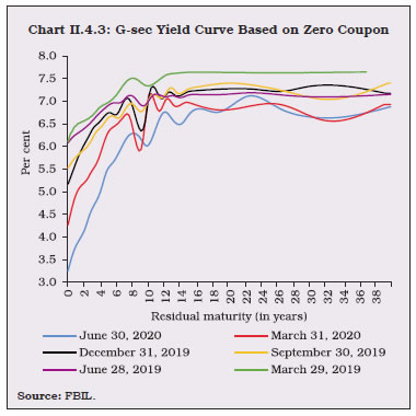
Box II.4.1
Impact of Special Operations by the Reserve Bank on Financial Markets Following Swanson, et al., (2011), a high frequency event study analysis was conducted around the announcement day of the Reserve Bank’s special OMOs in the nature of “Operation Twist (OT)”. One-day change in G-sec yields between the announcement day and the next trading day is calculated because the press releases of these announcements were posted on the Reserve Bank website after the close of financial markets. Statistical significance is measured relative to the unconditional standard deviation of the corresponding rate changes over similarly sized windows over a period of one year preceding the month of these announcements (Table 1). The results indicate that there was a statistically significant negative impact of the Reserve Bank’s OT announcements in December 2019 on 10-Year G-sec yields. | Table 1: Impact of Operation Twist Announcements on G-sec Yields on the Day of Announcement | | 1-day Change | 10-Year Benchmark | | 1 | 2 | | December 19, 2019 - December 20, 2019 | -13** | | December 26, 2019 - December 27, 2019 | -8* | | January 2, 2020 - January 3, 2020 | 0 | | January 16, 2020 - January 17, 2020 | 0 | | April 23, 2020 - April 24, 2020 | 0 | | June 29, 2020 - June 30, 2020 | -2 | | Cumulative, all announcements (in bps) | -23** | *: significant at 10 per cent **: significant at 5 per cent level.
Source: RBI staff estimates. | The dynamic impact of OT on the 10-year G-Sec yield is obtained by applying a Local Linear Projection (LLP) model which forecasts the path of the yield in response to the December 5, 2019 monetary policy announcement. The LLP model uses the overnight index swap (OIS) rates and the strategy expounded by Lloyd (2018) and Das et al. (2020), to filter ‘large surprise’ in monetary policy announcements between 2014 and 2019, and provides the impulse response of the yields to such ‘large surprises.’ Overall, twenty such ‘large surprise’ policies are identified between 2014 and 2019, including the policy announcement of December 5, 2019. The forecasted path is then compared with the observed path of the yield (Chart 1). The result suggests that the 10-year G-sec yield would have been higher without the two OT announcements in December 2019. The Reserve Bank first announced its intention to carry out LTRO in its Statement on Developmental and Regulatory Policies (February 6, 2020). The Reserve Bank made a total of eight announcements of LTRO till June 2020 out of which five were targeted LTRO announcements. The change in the yield of the securities selected under LTRO are analysed (Table 2). The results show that the cumulative impact of LTRO announcements was a reduction in 3-Year and 1-Year G-sec yields. | Table 2: Impact of LTRO on G-sec Yield | | Estimated Responses to Announcements (in bps) | 3-Year G-sec | 1-Year G-sec | | 1 | 2 | 3 | | 3-day change, Feb 5, 2020 - Feb 10, 2020 | -27.9* | -8.5 | | 1-day change, Feb 25, 2020 - Feb 26, 2020 | -5.3 | -1.9 | | 1-day change, Mar 16, 2020 - March 17, 2020 | 6.8 | 11.1* | | 2-day change, Mar 26, 2020-Mar 30, 2020# | -25.3* | -19.0* | | 1-day change, Mar 30, 2020-Mar 31, 2020# | -0.4 | -14.4* | | 1-day change, Apr 3, 2020 - Apr 7, 2020# | 8.2 | -3.5 | | 1-day change, Apr 15, 2020 - Apr 16, 2020# | -9.0 | -2.0 | | 2-day change, Apr 16, 2020 - Apr 20, 2020# | -37.6* | -23.8* | | Cumulative, all announcements (in bps) | -90.5* | -62.0* | *: significant 1 per cent level.#: Targeted LTRO dates.
Source: RBI staff estimates. | References: 1. Lloyd, S. P. (2018), 'Overnight Index Swap Market-based Measures of Monetary Policy Expectations', Bank of England Staff Working Paper No. 709. 2. Swanson, E. T., Reichlin, L., & Wright, J. H. (2011), 'Let’s Twist Again: A High-Frequency Event-Study Analysis of Operation Twist and Its Implications for QE2' [with Comments and Discussion], Brookings Papers on Economic Activity, 151-207. 3. Das, S., Ghosh, S., & Kamate, V. (2020), 'Monetary Policy and Financial Markets: Twist and Tango', Reserve Bank of India Bulletin, Volume LXXIV (8), 41-50. | II.4.14 FPI limits are revised on a half yearly basis under the medium-term framework (MTF)19, with the objective of ensuring a more predictable regime for investment by the FPI. Accordingly, investment limits for FPI in G-sec including State Development Loan (SDLs) were increased in a phased manner from ₹3,27,900 crore as on April 6, 2018 to ₹3,95,200 crore as on April 1, 2019. The limit was increased further to ₹4,29,500 crore as on October 1, 2019. During April-December 2019, FPIs made investment in G-secs and SDLs of ₹23,522 crore, while they pulled out ₹57,348 crore in Q4:2019-20, resulting in an overall net outflow during 2019-20. The outflow was pronounced in the fourth quarter, particularly in March 2020 that witnessed an outflow of ₹48,279 crore, in line with other emerging market economies (EMEs) hit by the outbreak of COVID-19. Therefore, FPI utilisation of total available limit (inclusive of investments in SDL) declined to 37.5 per cent on March 31, 2020 from 54.1 per cent a year ago. It was announced in the Union Budget 2020-21 that certain specified categories of G-sec would be open fully for non-resident investors apart from being available to domestic investors. Accordingly, in consultation with the government, a separate route, viz., the Fully Accessible Route (FAR) for investments by non-residents, including FPIs, in G-secs was introduced with effect from April 1, 2020. Five G-secs were specified as eligible for investment under the FAR, from the date on which the scheme comes into effect. In addition, all new issuances of G-secs of 5-year, 10-year and 30-year tenors from the financial year 2020-21 will be eligible for investment under the FAR as ‘specified securities’. 4. Corporate Debt Market II.4.15 Corporate bond yields largely tracked G-sec yields. The yield on 5-year AAA-rated corporate bonds softened during 2019-20, reflecting reduction in the policy repo rate, surplus systemic liquidity conditions, and the impact of special OMOs and LTRO auctions conducted during the latter part of the year. However, yields registered some uptick in March 2020 with the unfolding of distress in a major private bank and COVID-19. During the period March 12-25, 2020, turbulence in global financial markets and worsening of financial conditions resulted in a hardening of 5-year AAA-rated corporate bond yield by 72 bps. This was addressed by the announcement of various liquidity measures by the Reserve Bank on the back of a sizeable reduction in the policy rate. Overall, the 5-year AAA-rated corporate bond yield eased by 108 bps to 7.02 per cent during 2019-20. II.4.16 The risk premia or spread (5-year AAA-rated bond yield over 5-year G-sec yield) on bonds issued by public sector undertakings (PSUs), financial institutions (FIs) and banks; NBFCs; and corporates fell by 58 bps, 34 bps and 14 bps, respectively. The average daily turnover in the corporate bond market increased to ₹8,532 crore during 2019-20 from ₹7,587 crore a year ago (Chart II.4.4). II.4.17 Primary corporate bond issuances increased by 6.6 per cent to ₹6.9 lakh crore during 2019-20 as softening of yields encouraged corporates to mobilise higher resources from the corporate bond market, particularly public sector entities. Private placements remained the preferred choice for corporates, accounting for 97.8 per cent of total resources mobilised through the bond market. In order to provide an alternative source of financing for public sector entities at lower cost and help deepen bond markets by diversifying investor base with increased retail participation, the Government of India (GoI) launched the Bharat Bond Exchange Traded Fund (ETF) in December 2019 – the first ETF for corporate bonds in India – under which ₹12,395 crore were mobilised. Outstanding corporate bonds increased by 6.1 per cent y-o-y to ₹32.5 lakh crore or 16.0 per cent of GDP at end-March 2020. Investments by FPIs in corporate bonds decreased to ₹1.73 lakh crore at end-March 2020 from ₹2.19 lakh crore at end-March 2019. Consequently, utilisation of the approved limit by FPIs declined to 54.5 per cent at end-March 2020 from 75.9 per cent at end-March 2019. 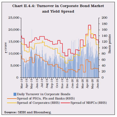 5. Equity Market II.4.18 The Indian equity market, which reached an all-time high on January 14, 2020, began to slide thereafter and trimmed its gains during 2019-20, especially after the outbreak of COVID-19. Volatility soared to unusually high levels. Overall, the BSE Sensex and the Nifty 50 plummeted by 23.8 per cent and 26.0 per cent, respectively, over end-March 2019. The India VIX, which captures short-term volatility of the Nifty 50, surged to 83.6 per cent on March 24, 2020 compared with 85.1 per cent during the GFC, before closing at 64.4 per cent on March 31, 2020 (Chart II.4.5). II.4.19 The BSE Sensex commenced the year with modest gains before declining during early May 2019 on concerns over weak corporate earnings and intensification of trade tensions between the US and China. However, prospects of a stable government and expectations of further monetary easing by the Reserve Bank buoyed market sentiment driving the BSE Sensex to 40,000 levels in June 2019. However, this rally proved transient as bearish sentiment gripped markets after a default by a housing finance company fuelled liquidity concerns in the NBFC sector in June 2019. II.4.20 The downtrend deepened in July 2019 over the Budget proposals such as (i) tax on super rich; (ii) buyback tax; and (iii) increase in minimum public shareholding in listed companies. Markets remained under pressure on negative cues from global equity markets, reporting of a borrowing fraud in a public sector bank, concerns over lacklustre corporate earnings results for Q1:2019-20, slow progress of monsoon and continued FPI outflows due to the proposed increase in tax surcharge for FPIs registered as non-corporates. The BSE Sensex declined marginally in August 2019, unsettled by adverse domestic developments such as tepid corporate earnings results for Q1:2019-20, lukewarm industrial activity and auto sales, and negative global cues, viz., political unrest in Hong Kong, debt default in Argentina and uncertainty over the US-China trade relations. However, the rollback of the super-rich tax on FPIs, front-loading of capitalisation of public sector banks and deferment of a hike in registration fees for automobiles provided some support to market sentiment. 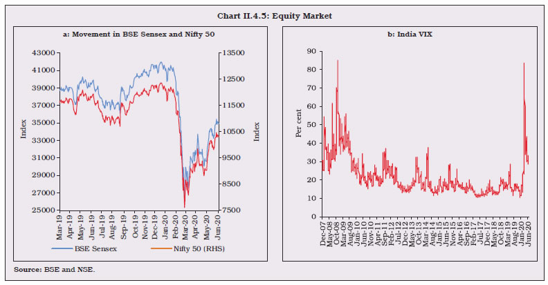 II.4.21 The BSE Sensex rose by five per cent on a single day on September 20, 2019 after the announcement of a reduction in the corporate tax rate. Subsequently, fresh optimism over the US-China trade negotiations and agreement on Brexit deal helped the BSE Sensex to reclaim 40,000 level on October 30, 2019. The bullish momentum gathered strength on growth boosting measures by the GoI, support to the Insolvency and Bankruptcy Code (IBC) amendment and approval for a partial credit guarantee scheme for public sector banks to purchase pooled assets from NBFCs. Furthermore, global tailwinds due to the US Fed’s dovish outlook, the US-China Phase-1 trade deal and Brexit-favouring UK election outcome aided the upswing. A slew of positive macroeconomic developments thereafter, including fall in global crude prices, recovery in industrial output in November, higher GST collections and expansion in manufacturing Purchasing Managers’ Index (PMI) for December, drove the BSE Sensex to close at a record of 41,953 on January 14, 2020. II.4.22 Markets wilted, however, under escalating geo-political tensions between the US and Iran, a weak domestic GDP growth outlook along with downward revision of India’s growth forecast for 2019-20 by the International Monetary Fund (IMF) and higher CPI inflation print for December 2019. The decline intensified on February 1, 2020 with the Sensex plunging by 988 points (2.4 per cent) as proposals in the Union Budget 2020-21 fell short of market expectations. However, markets made a V-shaped recovery on February 4, 2020 on the back of a sharp fall in crude oil prices and release of robust manufacturing PMI data for January 2020. Subsequently, the announcement of credit and liquidity enhancing measures on February 6, 2020 also supported market. This recovery, however, proved short-lived. II.4.23 Beginning February 20, 2020, fears over COVID-19 induced slowdown reverberated across the globe as equity markets both in advanced and EMEs, including in India, witnessed panic sell-offs. The BSE Sensex fell by 2,919 points (8.2 per cent) on March 12, 2020 following the declaration of COVID-19 as pandemic by the WHO. The market lost further ground with the BSE Sensex falling over 10 per cent during early hours of trading, attracting circuit breakers and suspension of trading for 45 minutes. A statement from SEBI indicating that the fall in the Indian stock indices has been significantly lower than in many other countries and assuring market participants of suitable and appropriate actions, if required, helped calm market nerves with the BSE Sensex ending on March 13, 2020 with a net gain of 1,325 points (4.0 per cent), the largest ever recovery in a single day. However, these gains could not be sustained as bearish sentiment returned on the back of continued moderation in global crude prices and growing worries over the impending recession. The Indian equity market breached the lower circuit bound for the second time in a month, with the BSE Sensex recording its biggest fall of 3,935 points (13.2 per cent) on March 23, 2020. Markets regained some lost ground thereafter amidst expectations of fiscal measures by the government, announcement of comprehensive monetary, liquidity and regulatory measures by the Reserve Bank including a sizeable reduction in policy rates on March 27, 2020. Overall, the BSE Sensex registered a decline of 23.1 per cent during March 2020. This sell-off in the equity market was accompanied by a surge in VIX from 23.2 per cent at end-February 2020 to a high of 83.6 per cent during March 2020 before closing at 64.4 per cent. However, it is observed that over the last few years, domestic institutional investors (DIIs) are increasingly emerging as a counter balancing force to FPIs during stress situation. During March 2020, when FPIs were net sellers to the tune of ₹62,434 crore, DIIs, led by MFs and insurance companies, were net buyers to the tune of ₹55,595 crore, thereby largely counter-balancing the withdrawal by FPIs. Further, the correlation between monthly net investments of MFs and FPIs during 2019-20 came out as high as -0.9, suggesting a strong counter balancing force during the time of FPI sell-offs. II.4.24 The market capitalisation of companies listed on BSE declined by 27 per cent to ₹113.5 lakh crore at end-March 2020 from ₹155.5 lakh crore at end-December 2019, before recovering to ₹129.4 lakh crore at end-April 2020. Hence, market capitalisation at end-March 2020 stood at 55.8 per cent of GDP as compared with 77.9 per cent at end-December 2019. II.4.25 Heightened volatility in domestic financial markets was caused by panic selling by FPIs (Box II.4.2). To comprehend the overall financial conditions, a Financial Conditions Index (FCI) was constructed using Principal Component Analysis on twelve indicators across different market segments. The values of the FCI above zero indicate higher-than-average levels of financial market stress/tightened financial conditions, while values below zero indicate lower-than-average levels of stress/loose financial conditions. The significant tightening of financial conditions as manifested in sharp correction in equity markets, widening of credit spreads and depreciation of the Indian rupee, is suggested by the FCI as well. Financial conditions eased subsequently in response to various liquidity measures undertaken by the Reserve Bank (Chart II.4.6). Box: II.4.2
India’s Financial Markets: Impact of COVID-19 The outbreak of COVID-19 impacted global financial markets and brought an abrupt tightening of financial conditions. In India, the stock market began to fall starting mid-February 2020 and plummeted thereafter with the declaration of COVID-19 as a pandemic by the WHO on March 11, 2020. Nifty 50 slumped by 38.4 per cent by March 23, 2020 from its peak of 12,362 on January 14, 2020 before making some recovery (Chart 1). The sectors that have been hit hardest include hotels, media, construction, power, auto, metals and banks, whereas telecom, pharmaceuticals, personal care, tea and coffee, petroleum, gas and IT have outperformed the overall market (Chart 2). 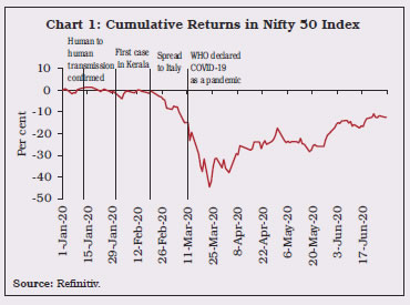
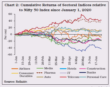 Financial conditions tightened across fixed income markets due to panic sell-offs by FPIs from EMEs, coupled with liquidation of positions by MFs to meet redemption pressures from investors, particularly those invested in funds with higher credit risk. This was reflected in widening of spread of G-sec and corporate bond yields over the policy repo rate (Chart 3). However, spread of 3-year and 5-year G-sec and corporate bond yields narrowed subsequently over the policy repo rate. Credit default swaps (CDS) premium of Indian banks dropped sharply from six-year highs on expectations that recent policy support would help lenders to avoid worse damage from the pandemic (Chart 4). 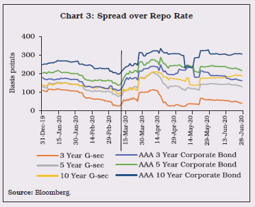
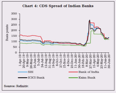
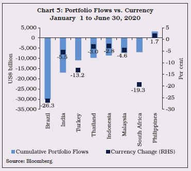
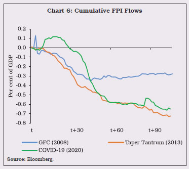 As bearish sentiment gripped markets, EMEs witnessed sharp reversal of capital flows with their currencies experiencing significant depreciations. India experienced one of the highest outflows amongst emerging market peers, but its currency performed relatively better (Chart 5), with the depreciation of the rupee being lower than at the time of the GFC and taper tantrum despite large outflows (Chart 6). References: 1. IMF (2020), 'Global Financial Stability Report', April. 2. Ramelli and Wagner (2020), 'Feverish Stock Price Reactions to COVID-19', CEPR Discussion Paper, No. DP14511. |
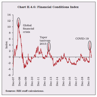
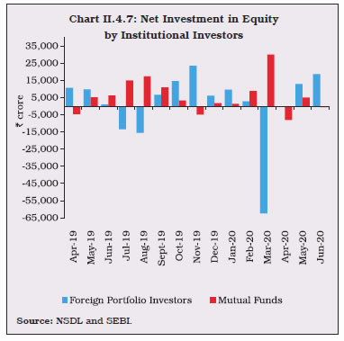 II.4.26 Net investment by DIIs, particularly MFs, provided support to the equity market during 2019-20. While MFs were net buyers to the tune of ₹91,160 crore, FPIs were net sellers of ₹6,204 crore, in the Indian equity market (Chart II.4.7). FPIs made net purchases of ₹63,509 crore during September 2019 to February 2020, but they made net sales of ₹62,434 crore during March 2020 as the spread of COVID-19 triggered flight to safety. Primary Market Resource Mobilisation II.4.27 The primary segment of the equity market witnessed increased activity during 2019-20. Resource mobilisation through initial public offers (IPOs), follow-on public offers (FPOs) and rights issues jumped more than four-fold to ₹76,382 crore during 2019-20. Of these, ₹21,323 crore were mobilised through 60 IPO/ FPO issues, out of which 46 issues amounting to ₹495 crore were listed on the Small and Medium Enterprises (SME) platform of the BSE and the NSE. Resource mobilisation through rights issues amounted to ₹55,059 crore mostly by telecom companies. Resource mobilisation through qualified institutional placement (QIP) also increased sharply to ₹51,216 crore in 2019-20 from ₹10,289 crore in 2018-19 (Appendix Table 5). II.4.28 Net resources mobilised by mutual funds declined by 20.4 per cent to ₹87,301 crore in 2019-20. Net resource mobilisation through equity-oriented schemes declined to ₹81,597 crore in 2019-20 from ₹1.1 lakh crore in 2018-19. Assets under management of equity-oriented mutual funds declined by 32.4 per cent to ₹6.0 lakh crore at end-March 2020 from ₹8.9 lakh crore at end-March 2019. 6. Foreign Exchange Market II.4.29 In the foreign exchange market, turnover in both merchant and the inter-bank segments of the spot and forward market mostly remained at the previous year’s levels, while the swap segment exhibited an increase in activity during the latter part of the year. II.4.30 The Indian rupee traded with a weakening bias, tracking other EME currencies during 2019-20, touching a then lifetime low against the US dollar in March 2020. While the depreciation of rupee was modest during H1:2019-20 – it depreciated by 2.31 per cent against the US dollar – mainly due to a sell-off in the equity market during July-August 2019 amidst concerns over escalating US-China trade tensions and tepid global growth. Thereafter, the rupee recovered some lost ground, tracking gains in the equity market following the announcement of corporate tax cuts. The rupee continued to extend the gains heading into H2:2019-20 on positive sentiment around growth boosting measures by the government and the trade truce between the US and China. However, the rupee came under intense pressure since then, triggered by flight to safety by FPIs on weakening of growth and COVID-19 concerns. It touched an all-time intra-day low of ₹76.29 on March 23, 2020. Although the Indian rupee depreciated by 8.88 per cent against the US dollar during 2019-20, it performed better than other EME currencies. (Chart II.4.8). 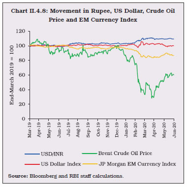 II.4.31 In tandem with movements in the nominal exchange rate of the rupee, the 36-currency nominal/real effective exchange rate (NEER/ REER) remained range-bound during 2019-20, barring a sharp depreciation in both 36-currency NEER and REER in August 2019 and March 2020. On average, the 36-currency NEER and REER appreciated by 0.9 per cent and 2.4 per cent, respectively, during 2019-20 on a y-o-y basis. II.4.32 Forward premia softened across the tenors during the year under the downward pressure exerted by the substantial increase in banking system liquidity. However, the near-term premia edged higher in the February-March period as rupee demand increased ahead of end-year closure of accounts. II.4.33 Going forward, financial market movements would hinge to a large extent on the progress made in containing the COVID-19 pandemic. Measures taken by the government and the central bank in addressing the macroeconomic and financial fallout of COVID-19 would also play an important role in shaping the behaviour of financial markets. II.5 GOVERNMENT FINANCES II.5.1 In 2019-20, general government finances deviated from budgetary targets. For the central government, the overshoot of 1.3 percentage points in its gross fiscal deficit (GFD) was mainly due to lower than budgeted tax collections, reflecting the growth slowdown as well as rationalisation of corporate tax rates. Thus, the central government took recourse to the escape clause under Section 4 (3) of the revised FRBM Act twice in 2019-20 – first, for its GFD being placed at 3.3 per cent of GDP in the budget estimates (BE) (0.2 percentage points above the glide path specified in 2018-19) on account of GST stabilisation and second, for the GFD overshooting to 3.8 per cent in its revised estimates (RE). As per provisional accounts (PA), however, the central government’s realised GFD reached 4.6 per cent. In the case of states, the consolidated GFD deviated from the budgeted level, again mainly on account of lower revenue collections20. II.5.2 Against this backdrop, sub-sections 2 and 3 present the position of central government finances in 2019-20 and 2020-21, respectively. Sub-sections 4 and 5 outline the developments in state government finances during 2019-20 and 2020-21, respectively. General government finances are discussed in sub-section 6. The final section sets out concluding remarks and some policy perspectives. 2. Central Government Finances in 2019-20 II.5.3 In 2019-20, the provisional accounts (PA) indicate that the central government’s GFD recorded a slippage of 1.3 percentage points from the target set in the Union Budget. Estimates for gross tax revenue in 2019-20 were brought down by ₹4.51 lakh crore vis-à-vis BE. On a year-on-year (y-o-y) basis, direct taxes declined by 7.7 per cent in 2019-20 (PA) as against a 13.4 per cent increase in 2018-19, whereas indirect tax growth decelerated to 1.7 per cent from 2.9 per cent a year ago. Although the shortfall in tax revenues was partially compensated by an increase in non-tax revenues, primarily due to transfer of excess reserves from the Reserve Bank21 and partial settlement of pending adjusted gross revenue (AGR) dues by telecom companies, they fell short of the RE. Moreover, only about half of the budgeted disinvestment target of ₹1.05 lakh crore was achieved. While capital expenditure was close to the budget target, revenue expenditure was curtailed to 96.0 per cent of the budgeted level, primarily through rollover of food subsidy. 3. Central Government Finances in 2020-21 II.5.4 The Union Budget 2020-21 attempts to balance the dual imperatives of providing countercyclical support to growth and charting a return to the FRBM’s prescribed fiscal deficit path (Table II.5.1). The consolidation in 2020-21 budget is to be achieved through higher non-tax revenue, led by spectrum auction and usage charges budgeted at ₹1.3 lakh crore. Moreover, non-debt capital receipts have also been budgeted higher, on the back of disinvestment receipts of ₹2.1 lakh crore, almost four times of what was realised in 2019-20 (Chart II.5.1). II.5.5 The implicit tax buoyancy of 2.0 in 2020-21 (BE) over 2019-20 (PA) is higher than the realised buoyancy of (-) 0.5 in 2019-20 (PA); this might also prove to be challenging (Chart II.5.2). | Table II.5.1: Central Government’s Fiscal Performance* | | (Per cent of GDP) | | Item | 2004-08 | 2008-10 | 2010-15 | 2014-15 | 2015-16 | 2016-17 | 2017-18 | 2018-19 | 2019-20 (RE) | 2019-20 (PA) | 2020-21 (BE) | | 1 | 2 | 3 | 4 | 5 | 6 | 7 | 8 | 9 | 10 | 11 | 12 | | Non Debt Receipts | 11.0 | 9.7 | 9.5 | 9.2 | 9.1 | 9.4 | 9.1 | 8.8 | 9.5 | 8.6 | 10.0 | | Gross Tax Revenue (a+b) | 10.7 | 10.4 | 10.2 | 10.0 | 10.6 | 11.1 | 11.2 | 11.0 | 10.6 | 9.9 | 10.8 | | a) Direct Tax | 5.1 | 6.0 | 5.7 | 5.6 | 5.4 | 5.5 | 5.9 | 6.0 | 5.8 | 5.2 | 5.9 | | b) Indirect Tax | 5.6 | 4.4 | 4.5 | 4.4 | 5.2 | 5.6 | 5.4 | 5.0 | 4.9 | 4.7 | 4.9 | | Net Tax Revenue** | 7.9 | 7.6 | 7.3 | 7.2 | 6.9 | 7.2 | 7.3 | 6.9 | 7.4 | 6.7 | 7.3 | | Non-tax Revenue | 2.2 | 1.8 | 1.8 | 1.6 | 1.8 | 1.8 | 1.1 | 1.2 | 1.7 | 1.6 | 1.7 | | Non Debt Capital Receipts | 0.9 | 0.3 | 0.4 | 0.4 | 0.5 | 0.4 | 0.7 | 0.6 | 0.4 | 0.3 | 1.0 | | Total Expenditure | 14.5 | 16.1 | 14.4 | 13.3 | 13.0 | 12.8 | 12.5 | 12.2 | 13.3 | 13.2 | 13.5 | | Revenue Expenditure | 12.1 | 14.4 | 12.6 | 11.8 | 11.2 | 11.0 | 11.0 | 10.6 | 11.6 | 11.6 | 11.7 | | Capital Expenditure | 2.4 | 1.7 | 1.8 | 1.6 | 1.8 | 1.8 | 1.5 | 1.6 | 1.7 | 1.7 | 1.8 | | Revenue Deficit | 2.0 | 5.0 | 3.5 | 2.9 | 2.5 | 2.1 | 2.6 | 2.4 | 2.5 | 3.3 | 2.7 | | Gross Fiscal Deficit | 3.5 | 6.3 | 4.9 | 4.1 | 3.9 | 3.5 | 3.5 | 3.4 | 3.8 | 4.6 | 3.5 | BE: Budget Estimates. RE: Revised Estimates. PA: Provisional Accounts.
*: GDP figures used in this table are on 2011-12 base, which are the latest available estimates. Going by the principle of using latest available GDP data for any year, GDP used for 2019-20 (RE) is the latest available Provisional Estimate (released on May 29, 2020). In view of this, the fiscal indicators as per cent of GDP given in this Table may at times marginally vary from those reported in the Union Budget Documents.
**: Net tax revenue represents gross tax revenue net of devolution to state governments.
Source: Union Budget Documents. | II.5.6 Total expenditure is budgeted to grow at a lower rate of 13.2 per cent in 2020-21 as compared with 16.0 per cent in 2019-20 (PA) due to a sharp deceleration in the growth of revenue expenditure from 17.0 per cent in 2019-20 to 11.9 per cent in 2020-21 (BE). The freeze in dearness allowance, as announced by the Union Government, and the compression under other heads of revenue expenditure will likely be offset by the increased expenditure requirement to fight COVID-19, including the increased interest expenditure due to higher volume of borrowings. Expenditure on major subsidies, viz., food, fuel and fertilisers, is budgeted to decline marginally to 1.0 per cent of GDP in 2020-21 from 1.1 per cent in 2019-20. Capital expenditure, on the other hand, is budgeted to grow at 22.4 per cent in 2020-21. The capital expenditure target for communications, however, has been budgeted five times higher in the Union Budget 2020-21 than in 2019-20 (RE), again a challenging task. An important goal of the Budget is reforms in the areas of labour, investment, coal and mining, which could revive economic activity and impart buoyancy to revenues. 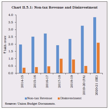
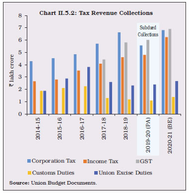 4. State Finances in 2019-20 II.5.7 As per the information available for 25 state governments, the consolidated fiscal position of states – in terms of the GFD-GDP ratio – deteriorated to 2.8 per cent in 2019-20 (RE) vis-à-vis BE of 2.3 per cent (Chart II.5.3). This deviation was mainly caused by the economic slowdown leading to lower revenue – both own and central transfers. Under own tax revenue, the decline was pronounced in states’ goods and services tax (SGST) and taxes on vehicles, which induced cuts in capital expenditure. Under revenue expenditure, allocation to development expenditure was increased, while non-development expenditure was reduced. The reduction in capital expenditure was largely reflected in reduced spending towards rural development22,23. 5. State Finances in 2020-21 II.5.8 For 2020-21, states budgeted a consolidated GFD-GDP ratio of 2.3 per cent, mainly through higher revenue and lower expenditure. The increase in revenue is expected from higher own tax revenue and devolution of tax. The reduction in expenditure is likely to be more under spending on education, social security and welfare, relief on account of natural calamities, other agricultural programmes and energy. While higher capital spending is budgeted in education, medical and public health, rural and urban development, spending on energy and transport is expected to be curtailed. COVID-19 poses a major fiscal challenge to states' budgets, especially as they are also using discretionary (pro-cyclical) tax policy such as hiking duties on petrol and diesel and increasing sales tax/VAT on alcohol to offset revenue losses. 6. General Government Finances II.5.9 Based on information of 25 states, the general government fiscal deficit increased from 5.4 per cent of GDP in 2018-19 to 6.5 per cent in 2019-20 (RE). Outstanding liabilities also increased to 70.4 per cent of GDP in 2019-20 (RE) from 67.5 per cent in 2018-19. In 2020-21, fiscal deficit and outstanding liabilities are budgeted at 5.8 per cent and 70.5 per cent of GDP, respectively (Appendix Tables 6 and 7). However, based on provisional accounts information, the general government fiscal deficit (including all states) is expected to deteriorate further to about 7.5 per cent in 2019-20. Thus, the fiscal gains achieved in the previous two years were reversed in 2019-20. A caveat is that most of the estimates for 2020-21 were worked out before the nation-wide lockdown. Given the shortfall in revenues – a direct fallout of subdued economic activity and increased expenditure requirement to fight the pandemic – the general government fiscal deficit and debt are likely to be materially higher than budgeted. II.5.10 In sum, the deterioration in major deficit indicators in 2019-20 may be attributed to tax revenue shortfall, both cyclical and structural. At the same time, a significant curtailment in expenditure was justifiably avoided in view of the economic slowdown, which got accentuated from the second half of 2018-19. Meeting the fiscal targets budgeted in 2020-21 has become even more challenging due to COVID-19, in view of containment measures and fiscal interventions for providing health infrastructure, helping vulnerable sections of the society and sector-specific relief measures. In this scenario, it is desirable to have a clear exit strategy with credible consolidation milestones and timelines in reworking the path towards fiscal rectitude in the coming years. II.6 EXTERNAL SECTOR II.6.1 Developments in the external sector during 2019-20 mirrored the unusual interplay of weak domestic and external demand, terms of trade gains from falling international crude prices and surges in net capital inflows. In the event, reserve buffers were strengthened, despite portfolio outflows towards the close of the year on widespread risk aversion triggered by the spread of COVID-19. II.6.2 Against this backdrop, sub-section 2 presents a brief overview of global economic and financial conditions followed by an analysis of merchandise exports and imports in sub-section 3. Sub-section 4 delves into the behaviour of invisibles. Together, sub-sections 3 and 4 unravel the movements in the current account balance during the year. Sub-section 5 dwells on net capital flows and movements in reserves. External vulnerability indicators are evaluated in sub-section 6, followed by concluding observations. 2. Global Economic Conditions II.6.3 In January 2020, the international environment began to improve with expectations of a US-China Phase 1 trade deal and an orderly Brexit. International organisations such as the IMF and the World Bank projected a recovery in global growth and trade for 2020 and 2021. The sudden outbreak of COVID-19 and swift contagion forcing the ensuing lockdown shattered this optimism. The loss of output, employment and life itself across 200 countries brought the global economy to standstill. This triggered a wave of downward revisions to global output growth, with the IMF projecting a contraction of world GDP by 4.9 per cent and trade volume by 11.9 per cent24 in 2020. The contraction in advanced economies (AEs) is projected to be more severe at 8.0 per cent while for the emerging markets and developing economies (EMDEs), it is milder at 3.0 per cent. The World Bank and the OECD also projected contraction in world GDP by 5.2 per cent and 6.0 per cent, respectively. In fact, the OECD projected a sharper contraction of 7.6 per cent, in case a second wave of COVID-19 hits before the year end. The impact on trade is expected to occur through various channels, including supply-chain disruptions, adoption of restrictive trade policies, volatility in international commodity prices, after-effects of lockdowns and lower demand resulting from the projected global recession. II.6.4 According to the WTO’s forecast of April 2020, world merchandise trade volume may plummet by 13 to 32 per cent during 2020. The WTO’s goods barometer index25 of May 2020 was at 87.6, its lowest value on record since the indicator was launched in July 2016. Prices of commodities dropped precipitously, creating pressure on commodity-exporting countries. Crude oil prices declined sharply due to demand compression caused by lockdowns coupled with a delay in production cuts by the Organisation of Petroleum Exporting Countries (OPEC) and its partners (OPEC plus). On the other hand, gold prices increased, reflecting safe-haven demand by investors amidst heightened global uncertainty. Inflationary pressures faced by EMDEs eased due to weaker demand and the sharp decline in oil prices. Global financial markets were buffeted by bouts of volatility amid investor concerns about downside risks to global growth accentuating towards the end of 2019-20. II.6.5 With the onset of the pandemic and growing fear of a deeper recession, global financial conditions tightened abruptly with a sharp fall in asset prices in EMEs as investors rushed to safety and liquidity. Currencies have fallen in the range of 5-25 per cent in Q4:2019-20 – faster than in the early months of global financial crisis (GFC). Central banks resorted to currency interventions and established swap lines with the US Fed and the ECB. Financial markets witnessed spikes in risk reversals and portfolio outflows of the order of US$ 95 billion from major EMEs between mid-January and end-March 2020 – more than thrice the amount experienced during the GFC. Several countries provided liquidity backstops to enable domestic banks to offer broad loan forbearance to borrowers. Central banks across the world have cut policy rates and pumped massive amounts of liquidity into markets through various conventional and unconventional measures, supplementing governments’ fiscal efforts to mitigate the fallout of COVID-19. 3. Merchandise Trade II.6.6 Global trade remained weak in 2019 due to trade tensions and slowing world economic growth. As per the WTO, global merchandise trade growth dropped to 0.1 per cent in volume terms in 2019, after growing by 2.9 per cent in 2018. India’s merchandise exports and imports contracted by 5.1 per cent and 7.8 per cent, respectively, during 2019-20, after three successive years of growth. Notwithstanding a marginal appreciation of the rupee in real effective terms – a measure of trade competitiveness – the estimated export volume remained more or less constant in 2019-20 vis-à-vis 2018-19, but falling export prices caused a decline in value terms. The deterioration in exports performance was broad-based – commodity groups constituting more than four-fifths of the export basket recorded lower values of shipments. The worsening profile of key export items, i.e., engineering products, gems and jewellery, petroleum products, rice, and cotton textiles was sector-specific, amplified by global developments (Chart II.6.1). Exports of items such as electronic goods, drugs and pharmaceutical and iron ore proved resilient and recorded expansion. II.6.7 The fall in exports of petroleum, oil and lubricants (POL) was largely driven by the softening of international crude oil prices, which plunged by 12.9 per cent during the year following the failure of the OPEC in reaching an agreement with Russia on production cuts and the resulting oversupply in global oil markets (Chart II.6.2). In volume terms, however, POL exports declined by 3.8 per cent. According to the Petroleum Planning and Analysis Cell (PPAC) of the Ministry of Petroleum & Natural Gas, crude oil processed by refineries witnessed a decline of 1.1 per cent (y-o-y), reflecting the closures of domestic refineries to meet the International Maritime Organisation (IMO) 2020 bunker fuel specifications as well as Bharat Stage (BS) VI emission norms which entailed supply of less polluting fuel across the country from April 1, 2020. 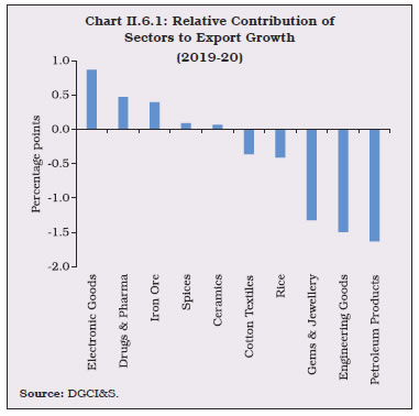
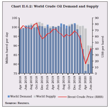 II.6.8 Rice exports declined due to non-basmati rice turning uncompetitive vis-à-vis other major exporters like China, Thailand, Vietnam and Pakistan, on account of the rise in minimum support price (MSP) of paddy. II.6.9 Gems and jewellery exports contracted by 10.8 per cent in 2019-20 on top of a decline of 3.1 per cent a year ago on account of the rise in import duty on precious stones and sluggish import demand from key destinations. Component-wise, the decline was mainly due to the slump in exports of pearl, precious and semi-precious stones. Destination-wise, Hong Kong, the UAE, the USA, Belgium and Israel, which account for 87 per cent of total gems and jewellery exports, registered a decline in demand. II.6.10 Engineering goods registered a decline of 5.9 per cent during 2019-20 as against a growth of 6.3 per cent a year ago. All major components, except electrical machinery and equipment (which accounted for around 11 per cent of total engineering goods exports), registered contraction. In particular, auto components and parts, ships, boats and floating structures, non-ferrous metals and products thereof, and industrial machinery were the key contributors to the decline. Destination-wise, the USA, which accounts for 16 per cent of India’s engineering goods exports, registered just 0.2 per cent growth. Germany, the UK, Nepal, Bangladesh and Mexico, which account for 17 per cent, registered a contraction in 2019-20. II.6.11 Exports of cotton textiles registered a decline of 10.6 per cent during 2019-20 as against a growth of 9.3 per cent a year ago. The contraction was mainly contributed by a decline of 29.1 per cent in the exports of cotton yarn. Bangladesh and China, which together accounted for around 43 per cent of these exports, posted double-digit declines. II.6.12 Electronic goods exports, which account for 3.7 per cent of total exports, grew continuously for 25 straight months since February 2018, driven by a rise in exports of telephone instruments, including smartphones (Chart II.6.3), and expanded by 32.5 per cent during 2019-20. Though India is not a significant player in the global smartphone market which is dominated by China, Vietnam and Hong Kong, it has the potential to play a crucial role in this market due to huge domestic demand and the rise of its digital economy. The UAE emerged as the largest destination for Indian mobile phone exports, followed by Russia, the US, Netherlands, South Africa and China (Chart II.6.4). 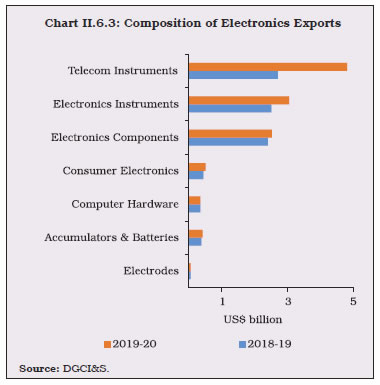 II.6.13 Drugs and pharmaceuticals exports grew by 8.1 per cent during 2019-20. COVID-19 has highlighted the concentration risks associated with China as India imports close to 70 per cent of active pharmaceutical ingredients (APIs), i.e., bulk drugs and intermediates, from China for manufacturing finished pharmaceutical products. Notably, India is not among the top 10 exporters or importers of medical products, and its medical exports are concentrated in medicines (pharmaceuticals) [Charts II.6.5 and II.6.6].
II.6.14 Iron ore exports picked up during 2019-20 on the back of a sharp increase in global iron ore prices, following production outages in Brazil. Nearly 80 per cent of total iron ore exports from India are shipped to China, which is the largest steel producer in the world. II.6.15 More than two-thirds of world trade passes through global value chains (GVCs) which straddle at least one border before final assembly. COVID-19 has posed challenges to GVCs as companies across the globe have significant exposure to Chinese GVCs (Box II.6.1). II.6.16 The slowdown in India’s merchandise imports that commenced in the second half of 2018-19 deepened further in 2019-20, with imports declining by 11.3 per cent in Q2:2019-20 as compared with an increase of 22.8 per cent in Q2:2018-19. Contraction in imports at the rate of 11.2 per cent set in during Q3:2019-20. COVID-19 accentuated the decline and imports fell by 9.8 per cent in Q4:2019-20. For the year as a whole, imports shrank by 7.8 per cent (Chart II.6.7). The retrenchment in imports during the year was spread across sectors, which constituted 95.4 per cent of the import basket, but mainly led by petroleum, oil and lubricants (POL), followed by pearls and precious stones, gold, coal, and transport equipment. In volume terms, however, imports remained stable in 2019-20 while import unit value declined by 8.6 per cent in 2019-20 as against a growth of 4.8 per cent a year ago. A few sectors, such as cotton, pulses, pharmaceutical products, and fruits and vegetables weathered the downturn and witnessed an expansion in imports during 2019-20. 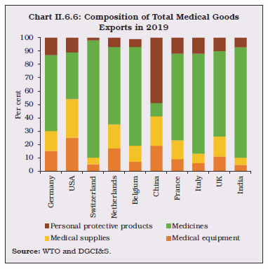
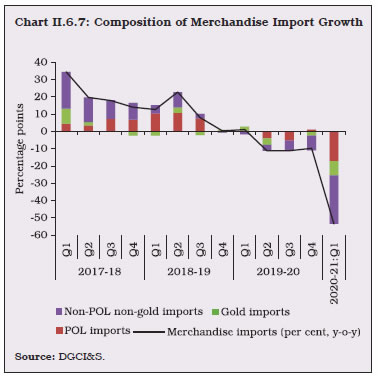
Box II.6.1
Global Value Chains in Pandemic Times World trade expanded rapidly on the back of the rise of global values chains (GVCs) after the 1990s, whose share in the world trade increased from around 38 per cent in 1970 to 41.6 per cent in 1990 and further to 51.8 per cent in 2008. Advancements in transportation, information and communication technologies and lowering of trade and tariff barriers encouraged manufacturers to extend production process beyond national boundaries (World Bank, 2020). According to the OECD, India’s foreign value-added content of exports increased to 25.1 per cent in 2011, from 18.8 per cent in 2005, although it declined to 16.1 per cent in 2016, lower than OECD and G-20 averages (25.3 per cent and 16.5 per cent, respectively). The decline is likely due in part to a shift towards local suppliers of intermediate inputs, particularly in the growing services sector. Recently, however, COVID-19 has revealed the fragility associated with GVCs, especially those associated with China, the US and Europe. Empirical findings suggest that a one per cent increase in GVC participation may boost per capita income levels by more than one per cent (World Bank, 2020). GVCs also have a more positive impact on productivity than conventional trade (IMF, 2019). Labour costs also play an important role in GVC participation (Ignatenko, Raei and Mircheva, 2019) - high labour costs in the exporting country decrease its competitiveness and thus limit its participation in GVC. Furthermore, the gains from participation in GVCs have not been distributed equally across and within countries. On the other hand, as the recent COVID-19 experience has shown, the concentration risk of GVCs in a single country can produce large global spillovers, impacting income, trade and investment. Indian industry’s integration with top 10 trading partners across 15 key sectors (which account for around three-fourths of India’s exports) can be measured through the Grubel-Lloyd Index (GLI)26. The following key points emerge: (i) India’s exposure to Chinese GVCs is somewhat limited (barring pharmaceutical and textiles) though China has a strong GVC presence in sectors like precision instruments, automotive and electrical machinery; (ii) India has a higher level of intra-industry trade integration with the Eurozone, followed by the US, Hong Kong, the UAE and Indonesia. Sector-wise and country-wise analysis suggests that intra-industry trade diversification may be strengthened with the Euro area, Indonesia and USA with regard to the automotive industry; with the Euro area, the USA, the UAE and Hong Kong for electrical machinery; and with Hong Kong, the USA, Indonesia and the UAE for precision instruments27 (Table 1). Table 1: India - Integration in GVC, by Sector, for Top 10 Major Trading Partners
(Grubel-Lloyd Index) | | Sector | China | Euro | USA | UAE | Saudi Arabia | Hong Kong | Switzer-land | Indo-
nesia | Korea | Singa-
pore | | 1 | 2 | 3 | 4 | 5 | 6 | 7 | 8 | 9 | 10 | 11 | | Petroleum Crude & Products | 0.081 | 0.097 | 0.111 | 0.182 | 0.023 | 0.014 | 0.000 | 0.103 | 0.896 | 0.169 | | Pharma Products | 0.417 | 0.412 | 0.089 | 0.003 | 0.000 | 0.079 | 0.131 | 0.730 | 0.447 | 0.665 | | Chemicals excluding Pharma | 0.193 | 0.475 | 0.342 | 0.144 | 0.286 | 0.285 | 0.328 | 0.162 | 0.280 | 0.214 | | Rubber/Plastics | 0.103 | 0.541 | 0.444 | 0.135 | 0.061 | 0.217 | 0.055 | 0.154 | 0.043 | 0.071 | | Leather Products | 0.158 | 0.171 | 0.048 | 0.008 | 0.002 | 0.082 | 0.166 | 0.563 | 0.311 | 0.641 | | Wood Products/Furniture | 0.049 | 0.388 | 0.128 | 0.296 | 0.008 | 0.053 | 0.263 | 0.090 | 0.200 | 0.121 | | Paper Products/Publishing | 0.085 | 0.161 | 0.128 | 0.115 | 0.044 | 0.089 | 0.025 | 0.057 | 0.016 | 0.167 | | Textiles and Apparel | 0.105 | 0.083 | 0.023 | 0.013 | 0.014 | 0.137 | 0.075 | 0.251 | 0.208 | 0.131 | | Gems & Jewellery | 0.019 | 0.462 | 0.527 | 0.419 | 0.008 | 0.288 | 0.005 | 0.004 | 0.021 | 0.528 | | Metals and Metal Products | 0.069 | 0.358 | 0.200 | 0.125 | 0.043 | 0.070 | 0.247 | 0.323 | 0.188 | 0.206 | | Office Mach/Machinery Various | 0.077 | 0.575 | 0.610 | 0.184 | 0.041 | 0.422 | 0.199 | 0.275 | 0.106 | 0.291 | | Communication Equipment | 0.021 | 0.576 | 0.785 | 0.136 | 0.006 | 0.237 | 0.275 | 0.379 | 0.024 | 0.118 | | Electrical Machinery | 0.055 | 0.597 | 0.530 | 0.466 | 0.016 | 0.331 | 0.256 | 0.306 | 0.076 | 0.188 | | Automotive | 0.122 | 0.706 | 0.207 | 0.029 | 0.000 | 0.315 | 0.146 | 0.243 | 0.168 | 0.160 | | Precision Instruments | 0.183 | 0.294 | 0.496 | 0.397 | 0.024 | 0.523 | 0.104 | 0.411 | 0.187 | 0.319 | | Source: RBI staff calculations. | Since several countries are looking to diversify away from China, this also provides a unique opportunity for India (Reynolds and Urabe, 2020; Chaudhary, 2020). Strengthening the domestic manufacturing sector’s participation in global value chains, liberalising trade, investments and FDI policy with regard to developing infrastructure (both hard and soft), providing reliable intellectual property rights for the international investor and implementing labour market reforms hold the key to India’s emergence as an important player in GVCs, going forward. References: 1. Ignatenko, A., Raei, F., & Mircheva, B. (2019), 'Global Value Chains: What are the Benefits and Why Do Countries Participate?' IMF Working Paper 19/18, International Monetary Fund, Washington, DC. 2. The World Development Report (2020), 'Trading for Development in the Age of Global Value Chains'. 3. Global Value Chain Development Report (2019), World Bank. 4. Global Economic Prospects (2020), World Bank. 5. UNCTAD (2020), 'Global Trade Impact of the Coronavirus (Covid-19) Epidemic', Division of International Trade and Commodities, UNCTAD Technical Note, March 4. 6. OECD (2018), 'Trade in Value Added: India'. | II.6.17 Imports of POL shrank by 7.4 per cent during 2019-20 on the back of a decline in international crude oil prices by 12.9 per cent (Chart II.6.8). Low global oil demand and expansion in production from non-OPEC countries such as the US and Canada limited upsides to international crude prices emanating from supply-side disruptions in Saudi Arabia, falling production of OPEC and the US sanctions on Iran and Venezuela. From January 2020, crude oil prices declined due to the Saudi-Russia price war and depressed demand. Venezuela and Iran, which together met 17.0 per cent of India’s crude oil imports in 2018-19, lost share in the aftermath of US sanctions. From June 2019, India stopped importing oil from Iran, compensating with stepped-up imports from other top suppliers such as Iraq, Saudi Arabia, the UAE and the US (Chart II.6.9). These developments created an upward price risk for India, as apart from being major sources of crude oil imports, Iran and Venezuela’s per barrel cost are lower than that of other suppliers, particularly the US. The estimated price of oil imported from Iran, Venezuela and the US was US$ 69, US$ 48 and US$ 70 per barrel, respectively, in 2019-20. 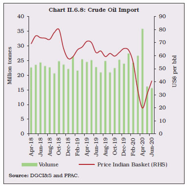
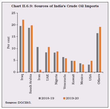 II.6.18 Gold imports at US$ 28.2 billion registered a decline of 14.2 per cent (y-o-y) in 2019-20. In volume terms, there was a significant contraction by 26.7 per cent in response to the rise in international gold prices by 15.8 per cent on safe haven demand (Chart II.6.10). The increase in gold import duty from 10 per cent to 12.5 per cent announced in the Union Budget 2019-20 also contributed to the decline in the volume of gold imports. II.6.19 Non-oil non-gold imports started contracting from Q4:2018-19, and the intensity of contraction deepened further during 2019-20. Among non-oil non-gold imports, pearls and precious stones, coal and chemical were major contributors to the deterioration (Chart II.6.11). A fall in coal imports by 14.2 per cent during 2019- 20 was driven by a sharp slump of 29.2 per cent in international coal prices. In volume terms, coal imports registered a modest growth of 4.6 per cent during the year. II.6.20 Imports of transport equipment contributed to the decline in capital goods imports. These imports were mainly pulled down by sectors such as ships, boats and floating structures, automobile parts and components, and railway equipment, mirroring subdued domestic demand conditions. China, Germany and the US accounted for about 42 per cent of India’s automobile parts and component imports. Imports of pearls and precious stone at US$ 22.5 billion contracted by 17.1 per cent in 2019-20 as imports from trading partners accounting for 89.2 per cent of India’s total imports of pearls and precious stones registered negative growth. Within pearls and precious stones, the decline was driven by a fall in the import of diamonds by 17.7 per cent (y-o-y) in 2019-20, the latter driving a decline in exports shipment of diamonds by 21.3 per cent (y-o-y) during the year. 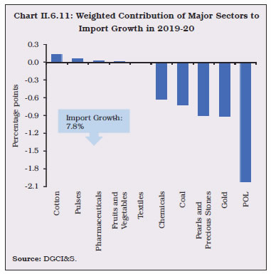 II.6.21 The pharmaceutical sector is a major contributor to India’s import growth. Medicinal and pharmaceutical products imports at US$ 6.5 billion registered a growth of 1.6 per cent (y-o-y) in 2019-20. Within this segment, imports of bulk drugs, intermediates and drug formulation together accounted for 88 per cent of pharmaceutical imports in 2019-20. India’s imports from China were as high as 68.0 per cent of its total bulk drugs and intermediates imports during this period. II.6.22 As the decline in imports was much larger than in exports during 2019-20, the merchandise trade deficit narrowed by US$ 23.1 billion to US$ 160.9 billion from US$ 184.0 billion a year ago, reflecting both subdued domestic economic activity and lacklustre export performance (Chart II.6.12). 4. Invisibles II.6.23 Net receipts from invisibles, reflecting cross-border transactions of services, income and transfers, increased during 2019-20, albeit at a slower pace than a year ago (Appendix Table 8). The growth in exports of software services and remittances receipts from overseas Indians boosted net invisible receipts which financed 84 per cent of the trade deficit during 2019-20 – higher than 68 per cent a year ago. II.6.24 India’s net export of services recorded a broad-based improvement across all sub-sectors, barring transportation, insurance and communication services (Chart II.6.13). Software services exports expanded at a quicker pace despite higher rejection rate of H-1B visa applications filed by Indian IT services firms in the US. Major IT companies secured multi-year IT services contracts and strategic deals in overseas markets. They also accelerated efforts towards new technologies such as artificial intelligence, machine learning, cloud computing and big data analytics to support their customers’ enterprise-wide transformation initiatives. 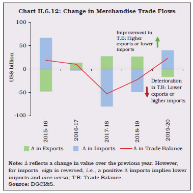
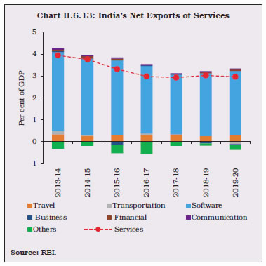 II.6.25 Net receipts from travel recorded double digit growth during 2019-20, reflecting the lower growth of payments on outbound travel, even though the tourist arrivals from high-income countries (except the US) were lower than a year ago. Reflecting the impact of the global spread of COVID-19, arrival of foreign tourists at 3.28 lakh recorded a contraction of 66.2 per cent on y-o-y basis in March 2020 which led to decline in tourist arrivals during 2019-20 by 3.8 per cent.28 Sluggish domestic economic activity and travel restrictions due to COVID-19 impacted outbound tourists from India, resulting in slower growth in travel payments (1.4 per cent) as compared with 11.2 per cent a year ago. II.6.26 Inbound remittances from Indians working abroad grew for the third consecutive year in 2019-20, though at a slower pace. Subdued remittance flows largely reflected weaker growth in AEs and lower crude oil prices weighing on incomes of oil producing Gulf countries. Nevertheless, India was the largest recipient, with a share of 11.3 per cent in global remittances in 2019. According to the World Bank estimate, the average cost of sending remittances to India decreased from 5.6 per cent in 2018-19 to 5.3 per cent in 2019-20 and remained significantly lower than the global average of 6.8 per cent.29 II.6.27 Under the income account, net cross-border income payments associated with the production and ownership of financial and other non-produced assets were lower during 2019-20 than in the preceding year. The decline was attributable mainly to a lower net outgo on account of investment income, which consists of dividends and withdrawals from income of quasi-corporations, reinvested earnings, and interest. Notwithstanding higher payments on debt and non-debt liabilities of the economy on account of foreign investments and external commercial borrowings, net outgo declined as interest earnings on foreign currency assets and dividend earnings of Indian FDI enterprises abroad increased over the preceding year. II.6.28 With the current account balance turning from deficit to surplus in Q4, the current account deficit (CAD) for the year narrowed to 0.9 per cent of GDP from 2.1 per cent in 2018-19 as the merchandise trade deficit contracted, reflecting the terms of trade gains accrued from lower commodity prices for crude oil, coal and fertilisers, and a contraction in import volumes (Charts II.6.14 and II.6.15).
5. External Financing II.6.29 In the financial account, all major sources of foreign capital increased. Net capital inflows were more than sufficient to finance the lower CAD and, therefore, this led to a large accretion to foreign exchange reserves in 2019-20 (Chart II.6.16). On a BoP basis (excluding valuation effect), forex reserves increased by US$ 59.5 billion in 2019-20 after a depletion of US$ 3.3 billion in 2018-19 (Box II.6.2). 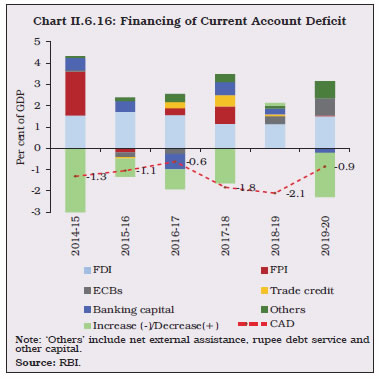
Box II.6.2
Capital Flows and Foreign Exchange Reserves:
An Analytical Perspective on Absorptive Capacity of the Domestic Economy The juxtaposition of the recent slowdown in domestic growth and surge in capital inflows leading to historically high build-up of reserves has brought into focus the question of the economy’s absorptive capacity – how much foreign capital can be effectively used by the economy for boosting growth, productivity and development (RBI, 2002). The issue assumes special relevance because foreign capital is generally seen to be beneficial to an economy; however, if it is not absorbed into the real economy to finance investment, it can possibly lead to upward pressure on the exchange rate, overheating of the economy and asset price bubbles. In countries with limited absorptive capacity, net capital flows greater than the funding needs of the CAD can lead to large accretions in foreign exchange reserves which are deployed outside the economy without realising benefits in terms of higher real consumption and investment. In other words, lack of absorptive capacity may constrain the growth-augmenting role of foreign capital. The absorptive capacity of an economy is generally constrained by lack of domestic demand; the scarcity of complementary factors of production such as skilled labour, technology, management and intermediate production inputs; and lack of institutional development. Incidentally, capital flows can be associated with higher growth only when the negative impact of their volatility on output and consumption is controlled for (World Bank, 2001). In the case of India, almost half of net capital flows (average of 2.7 per cent of GDP during 2013-14 to 2019-20) were accumulated as reserves (1.3 per cent of GDP) on the back of insufficient absorptive capacity in the domestic economy. Even though higher CAD (due to higher trade deficit) absorbed foreign capital flows during the post-GFC period (2009-10 to 2012-13), the quality of imports was characterised by unproductive gold imports and higher international crude oil prices rather than growth-inducing non-oil non-gold imports. In the post-taper tantrum phase of 2013-14 to 2019-20, net capital flows (as a ratio to GDP) were lower but exceeded the modest level of CAD, caused by lower crude oil prices and sharp moderation in growth in non-oil non-gold imports (i.e., average 2.4 per cent during 2013-14 to 2019-20 vis-à-vis 12.0 per cent during 2009-10 to 2012-13). Besides structural factors, low growth in recent years mainly due to subdued domestic demand has also constrained the capacity of the economy to absorb capital inflows. A vector error correction model using data for period 1997-98:Q1 to 2019-20:Q4 shows that oil import volume (both crude and products) has the largest growth-inducing impact, followed by capital goods and non-oil non-gold imports (Table 1). Imports with a good mix of capital goods, therefore, may not only enhance the domestic absorptive capacity but will also add to growth by ensuring productive use of foreign capital. To sum up, absorption of foreign capital is crucial for economic growth. It is the quality of CAD which matters in enhancing the absorptive capacity of the economy through growth-inducing imports. Further structural reforms backed by improved quality of CAD, therefore, would help the country lift the potential and sustain growth. Table 1: Growth inducing Impact of Imports
(Dependent Variable: Real GDP) | | Import | Error correction term | Long-run effect | | 1 | 2 | 3 | | Oil (crude and products) | -0.06** | 1.02* | | Non-oil non-gold# | -0.04* | 0.56* | | Capital goods# | -0.02*** | 0.81* | | Gold | No long-run relationship^ | #: Estimate based on period 2001-02: Q1 to 2019-20: Q4.
^: No cointegrating relationship found based on the Johansen test.
*, ** and ***: Indicate statistical significance at 1, 5 and 10 per cent, respectively.
Note: 1. All variables are in log form and estimates checked for Vector Error Correction Residual Serial Correlation and their normality. Optimal number of lags used is 4.
2. Estimates for imports of oil and gold are based on actual volumes reported by DGCI&S while non-oil non-gold imports and capital goods imports were deflated by UVI of India’s imports available under UNCTAD database.
Source: RBI staff calculations. | References: 1. Grenville, Stephen (2008), 'Central Banks and Capital Flows', ADBI Discussion Paper No. 87, Asian Development Bank Institute: Tokyo. 2. World Bank (2001), 'International Capital Flows and Economic Growth', Global Development Finance 2001, Chapter 3. 3. Reserve Bank of India (2002), Report on Currency and Finance. | II.6.30 Foreign direct investment (FDI) remained the predominant source of external financing, as in the preceding year. In both gross and net terms, FDI flows in 2019-20 were well above their respective levels in 2018-19 (Table II.6.1). Despite a slowdown in the global economy and growing global investment concerns due to disruptions in supply chains, India was able to sustain the pace of FDI in 2019-20 and was the 9th largest recipient country globally in 2019.30 Sustained business reforms in the areas of starting business, construction permits and insolvency resolution under the Insolvency and Bankruptcy Code (IBC) helped India gain 14 places and move to the 63rd position in the World Bank’s ease of doing business index (2020)31, from 77th position a year ago. According to the World Bank, India was one of the world’s top 10 most improved countries in terms of doing business for the third consecutive year. Most of FDI equity flows went to the services sector, including communication services, retail and wholesale trade, financial services, computer and business services and the manufacturing sector. Singapore and Mauritius remained the major source countries, accounting for about 50 per cent of total FDI flows in 2019-20, followed by the Netherlands, the Cayman Islands, the US and Japan (Chart II.6.17 and Appendix Table 9). | Table II.6.1: Foreign Direct Investment Inflows | | (US$ billion) | | Item | 2017-18 | 2018-19 | 2019-20 (P) | | 1 | 2 | 3 | 4 | | 1 Net FDI (1.1 - 1.2) | 30.3 | 30.7 | 43.0 | | 1.1 Net Inward FDI (1.1.1 - 1.1.2) | 39.4 | 43.3 | 56.0 | | 1.1.1 Gross Inflows | 61.0 | 62.0 | 74.4 | | 1.1.2 Repatriation/Disinvestment | 21.5 | 18.7 | 18.4 | | 1.2 Net Outward FDI | 9.1 | 12.6 | 13.0 | P: Provisional
Source: RBI. | II.6.31 Apart from equity investments, there was a substantial increase in the inter-corporate debt of FDI companies, which covers the borrowing or lending between affiliated direct investment enterprises. A simplification of the policy framework for external commercial borrowings (ECBs) since January 2019, allowing all entities that are eligible for FDI to raise ECBs and other relaxations such as expansion of scope of end-use of resources led to increased FDI flows of US$ 8.3 billion in 2019- 20, triple the level a year ago. 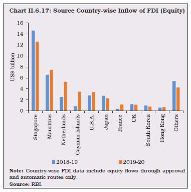 II.6.32 Outward direct investment by Indian entities also remained robust as Indian entities continued to expand their overseas business operations. Outward FDI was mainly in the form of equity and loans to subsidiaries/ affiliated enterprises, primarily to Singapore, the US, the UK, Mauritius, Switzerland and the Netherlands, which accounted for 75 per cent of total overseas investments during the period. Most of these investments were made in the business services, manufacturing and restaurants and hotels sector. II.6.33 Foreign portfolio investment (FPI) flows have remained volatile since the beginning of 2019-20 on account of multiple headwinds. Net FPI outflows under the general route were US$ 7.1 billion in 2019-20. After robust inflows in Q1:2019-20, FPIs undertook sell-offs in the equity segment in July 2019 on account of the domestic slowdown, particularly the auto sector, and the super-rich tax surcharge announced in the Union Budget. Outflows reversed, however, with the rollback of the tax surcharge and the corporate tax rate cut in September 2019. Monetary easing by major central banks and the US-China Phase 1 trade deal also supported FPI inflows in Q3:2019-20. However, an unprecedented wave of global risk aversion arising from the fear of global recession in the wake of COVID-19 and the ongoing crude oil price war between Saudi Arabia and Russia, triggered risk-off sentiments among global investors leading to net sell-offs of US$ 16.0 billion in Q4:2019-20 (Chart II.6.18). Nearly 70 per cent of the FPI outflows were from the banking and other financial services, software, oil and gas, and automobiles and auto components (Chart II.6.19). Country-wise, the composition of assets under custody as at end-March 2020 shows continued dominance of US-based foreign portfolio investors, followed by those operating through Mauritius, Luxembourg and Singapore. The Voluntary Retention Route (VRR), introduced to encourage long-term FPI in the debt market, however, attracted US$ 8.6 billion by end-March 2020. 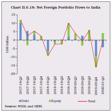
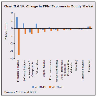 II.6.34 Various policy measures were undertaken during 2019-20 to expand investment opportunities and impart confidence to foreign investors: (i) increase in the statutory limit for FPI investment from 24 per cent to sectoral foreign investment limit with the option for corporates to limit it to a lower threshold; (ii) permitting FPIs to subscribe to listed debt securities issued by real estate investment trusts (ReITs) and infrastructure investment trusts (InvITs); and (iii) rationalisation of KYC norms for foreign investors. The Reserve Bank also introduced a slew of measures to encourage foreign inflows, which included (i) hike in the short-term investments by FPIs from 20 per cent to 30 per cent of the total FPI investment in central government securities (including Treasury Bills) or state development loans (SDLs); (ii) increase in investment cap under VRR scheme to ₹1,50,000 crore from ₹75,000 crore; (iii) flexibility to transfer investment under the general investment limit to the VRR scheme; and, (iv) expansion of the scope of instruments for investments under VRR to include exchange traded funds investing only in debt instruments. For 2020-21, the FPI limit in the domestic corporate bond market has been further raised from 9 per cent to 15 per cent of total outstanding stock of corporate bonds. Notwithstanding several confidence building measures and enhancement of FPI limits, FPI activity in 2019-20 was largely influenced by global developments. Utilisation of FPI limits dipped to 37.5 per cent in the government debt market (both G-sec and SDLs) and 54.5 per cent in the corporate debt market by end-March 2020 from 54.0 per cent and 75.9 per cent, respectively, a year ago. II.6.35 FPI outflows from the domestic capital market tracked the reversal of portfolio flows in major EMEs. In fact, FPI outflows from EMEs in Q4:2019-20 were the largest ever in any phase of flight to safety, including the Global Financial Crisis (GFC) (Chart II.6.20). II.6.36 Among other forms of financial flows, ECBs32 to India at US$ 21.7 billion in 2019-20 increased substantially from US$ 9.8 billion last year (Chart II.6.21). Ample global liquidity and a favourable overseas interest rate environment, along with various ECB liberalisation measures undertaken by the Reserve Bank to ease financial conditions, facilitated the access of domestic entities to global markets. The Reserve Bank allowed (i) ECBs with a minimum maturity of 10 years for working capital and general corporate purposes; (ii) ECBs with a minimum maturity of 7 years for repayment of rupee loans availed domestically for capital expenditures and minimum maturity of 10 years for non-capital expenditures; (iii) non-banking finance companies (NBFCs) to avail ECBs for on-lending for the same purposes as above; and (iv) ECBs with a minimum maturity of 7 years for rupee loans availed domestically for capital expenditure in manufacturing and infrastructure sector if classified as Special Mention Accounts (SMA-2) or Non-performing Assets (NPAs) under any one-time settlement with lenders. The favourable impact of these measures was reflected in higher utilisation of ECBs – 75 per cent of approvals in 2019-20 were utilised for on-lending or sub-lending, rupee expenditure on local capital goods, refinancing of rupee loans, working capital, infrastructure development and import of capital goods (Chart II.6.22). While rupee denominated loans and rupee denominated bonds (RDBs) accounted for 7.1 per cent of the agreement amount, 56.7 per cent (other than rupee denominated bonds/loans) was hedged in 2019-20 as compared with 45.6 per cent a year ago. Higher repayments relative to fresh disbursals, however, led to net outflows of US$ 1.8 billion in RDBs as against inflows of US$ 0.8 billion a year ago. After marginal net inflows in Q1, short-term trade credit declined in subsequent quarters as demand for fresh disbursals, both buyers’ and suppliers’ credit, moderated with slowdown in merchandise trade activity. Trade credit was primarily availed by domestic companies to finance imports of crude oil, coal, copper and gold, which together accounted for around 45 per cent of the total short-term trade credit raised during the period. 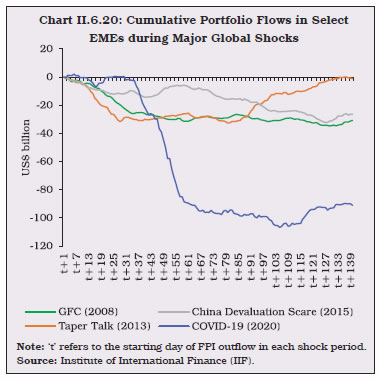
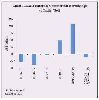
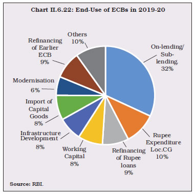 II.6.37 Net flows into non-resident deposit account declined by 17 per cent in 2019-20 as deposits under the Non-Resident (External) Rupee (NRE) accounts, which accounted for the bulk of the inflows, declined sharply. Softening of term deposit rates and expectations of further depreciation of rupee amidst global uncertainties partly moderated flows into this account. Among the other two accounts, deposits in Non-Resident Ordinary Rupee (NRO) accounts and the Foreign Currency Non-Resident (Banks) [FCNR (B)] accounts remained at the previous year’s level (Table II.6.2). 6. Vulnerability Indicators II.6.38 At end-March 2020, India’s external debt increased by US$ 15.4 billion (i.e., 2.8 per cent) from its level at end-March 2019, primarily on account of commercial borrowings. The increase in external debt was partially offset by valuation gains of US$ 16.6 billion resulting from the appreciation of the US dollar against Indian rupee and major currencies (such as euro and SDR). Excluding the valuation effect, the increase in external debt would have been US$ 32.0 billion instead of US$ 15.4 billion. Commercial borrowings remained the largest component of external debt, with a share of 39.4 per cent, followed by non-resident deposits (23.4 per cent) and short-term trade credit (18.2 per cent). As a ratio of GDP, external debt increased from 19.8 per cent at end-March 2019 to 20.6 per cent at end-March 2020. Notwithstanding an increase in external debt, other debt- and reserve-related indicators of external vulnerability improved. The share of short-term debt (on both original and residual maturity basis) in total debt declined. Similarly, foreign exchange reserve cover of imports and short-term debt (on both original and residual maturity basis) improved during the year, mainly reflecting the sizeable accretion in reserves. The latter also led to India’s net international investment position (NIIP) improving by US$ 57.6 billion (i.e., fall in net claims of non-residents on India) during the same period (Table II.6.3, and Appendix Table 1). | Table II.6.2: Flows under Non-Resident Deposit Accounts | | (US$ billion) | | | 2017-18 | 2018-19 | 2019-20 | | 1 | 2 | 3 | 4 | | 1. Non-Resident External (Rupee) Account | 7.1 | 7.3 | 5.6 | | 2. Non-Resident Ordinary Account | 1.5 | 1.9 | 2.0 | | 3. Foreign Currency Non-Resident (B) Account | 1.0 | 1.1 | 1.1 | | Non-Resident Deposits (1+2+3) | 9.7 | 10.4 | 8.6 | | Source: RBI. | II.6.39 Robust capital inflows, particularly during Q1 to Q3 of 2019-20, led to an accretion to the foreign exchange reserves, which reached a historic high of US$ 487.2 billion as on March 6, 2020. Consequent upon the 6-month US dollar sell/buy swap auction undertaken twice by the Reserve Bank in March 2020 to provide liquidity to the foreign exchange market and valuation losses caused by a sharp appreciation of the US dollar against major currencies, foreign exchange reserves, however, dipped to US$ 477.8 billion as at end-March 2020. | Table II.6.3: External Vulnerability Indicators (End-March) | | (Per cent, unless indicated otherwise) | | Indicator | 2013 | 2018 | 2019 | 2020 | | 1 | 2 | 3 | 4 | 5 | | 1. External Debt to GDP ratio | 22.4 | 20.1 | 19.8 | 20.6 | | 2. Ratio of Short-term Debt (original maturity) to Total Debt | 23.6 | 19.3 | 20.0 | 19.1 | | 3. Ratio of Short-term Debt (residual maturity) to Total Debt | 42.1 | 42.0 | 43.4 | 42.4 | | 4. Ratio of Concessional Debt to Total Debt | 11.1 | 9.1 | 8.7 | 8.6 | | 5. Ratio of Reserves to Total Debt | 71.3 | 80.2 | 76.0 | 85.5 | | 6. Ratio of Short-term Debt (original maturity) to Reserves | 33.1 | 24.1 | 26.3 | 22.4 | | 7. Ratio of Short-term Debt (residual maturity) to Reserves | 59.0 | 52.3 | 57.0 | 49.5 | | 8. Reserves Cover of Imports (in months) | 7.0 | 10.9 | 9.6 | 12.0 | | 9. Debt Service Ratio (debt service to current receipts) | 5.9 | 7.5 | 6.4 | 6.5 | | 10. External Debt (US$ billion) | 409.4 | 529.3 | 543.1 | 558.5 | | 11. Net International Investment Position (NIIP) (US$ billion) | -326.7 | -418.5 | -436.9 | -379.3 | | 12. NIIP/GDP ratio | -17.8 | -15.9 | -15.9 | -14.0 | | 13. CAD/GDP ratio | 4.8 | 1.8 | 2.1 | 0.9 | | Source: RBI and Government of India. | II.6.40 To sum up, India’s balance of payments in 2019-20 reflected muted domestic activity, but capital flows were robust, which engendered a large accretion to foreign exchange reserves. Improvement in major external vulnerability indicators occurred during the year, which should help mitigate spillovers from external shocks. The ensuing year is likely to be challenging due to a highly uncertain global trade and investment environment, and extreme fear and uncertainty about the intensity and spread of COVID-19. While terms of trade gains may provide some respite, the outlook is uncertain for exports, remittance inflows and the tourism sector. While companies may put their IT expansion plans on hold and cut back their overall IT spending, there could be pockets of opportunity for software and related services for Indian IT companies due to an increase in demand and usage for certain IT-enabled services by consumers and companies impacted by the pandemic. The prospects for capital flows face uncertainty due to their sensitivity to shifts in the global macroeconomic outlook. Going forward, the effectiveness of policy measures undertaken to address COVID-19 related stress is also likely to play a critical role in preserving the resilience of India’s external sector.
|