J. K. Khundrakpam and Rajiv Ranjan*
Employing an inter-temporal model on a constructed private consumption series, the paper finds that the current account balance in India during 1950-51 to 2005-06 is inter-temporally solvent. This is primarily a reflection of the developments that have taken place during the post-reform period, when restrictions on capital flows have been significantly liberalised. We do find some evidence of asymmetry between capital flows, which is on expected lines as restrictions on capital outflows from India are more than those on inflows to India. The study finds that the optimal current account balance has been larger than the actual current account balance. This is intuitively appealing as there were severe foreign exchange restrictions in the pre-reform period which restricted the smoothing of private consumption up to the optimal level. With further liberalisation of capital flows, both inflows and outflows, it would be possible for agents to further smoothen their consumption to desired optimal level, allowing scope for higher current account deficit to attain potentially higher growth.
JEL Classifications : E21, F32, F41
Keywords : Current account, Consumption-smoothing, Inter-temporal
Introduction
The last two to three decades have seen a shift in the thinking of policy makers and economists on the current account balance towards an inter-temporal model with consideration on long-term sustainability (Frenkel and Razin, 1987; Ghosh and Ostry, 1995; and Obstfeld and Rogoff, 1996). The model is based on the permanent income hypothesis where consumption expenditure of agents depends upon the expected permanent income. When the current income fluctuates, the current level of saving would also correspondingly fluctuate in order to maintain the level of consumption. Extended in the context of a small open economy, fluctuation in current income translates into borrowing or lending from the international markets i.e., movement of capital, to smooth out consumption. Thus, inter-temporal consumption optimisation behavior of agents predicts the desired level of capital flows to meet the resulting current account balance. Therefore, if the saving and investment decisions of agents are optimal, the resulting current account balance is also optimal and inter-temporally solvent, irrespective of whether it is in deficit, surplus or balanced.
* The authors are Directors in the Department of Economic Analysis and Policy. These are strictly the personal views of the authors.
This approach to analysing current account balance has a number of policy implications. First, if the current account balance is the outcome of optimising behavior of agents in the economy, it should not be a matter of concern for the policy makers since there will not be any unsustainable accumulation of foreign liabilities/assets. Second, the current account balance need not necessarily be the result of structural imbalances, but the outcome of economic agents’ response to temporary change in government expenditure or investment, which may not require policy initiatives such as exchange rate variation to correct the imbalance. Third, the observed current account balance may point toward the required growth of the economy in future, indicating either a higher growth to repay borrowed foreign savings or a possible lower growth while receiving its savings lent to foreigners. Fourth, when there are controls on capital flows, the model allows testing the effectiveness of these controls and check whether there are any avoidable welfare losses and potential growth foregone due to capital controls. Fifth, technically solvent current account balance does not guarantee its sustainability as lenders perception can change and raise doubts on the debtor country’s ability to meet its obligations particularly when restrictions on capital flows inhibits optimisation and there are unforeseen external shocks.
In the cross-country context, the empirical validity of inter-temporal model of current account balance, however, has been diverse and ambiguous. Otto (1992), Ghosh (1995) and Nason and Rogers (2003) rejects the validity of the model in the context of Canada. Similarly, Milbourne and Otto (1992), Guest and McDonald (1998) and Cashin and McDermott (1998a, 1998b) find that the model does not hold with Australian data.
In contrast, a number of studies have found the validity of model in several countries. They include: Otto (2003) for Australia during 1980 to 2000; Ghosh and Ostry (1995) in two-thirds of the 45 sample countries including India during 1960 to 1990; Agenor, et al (1999) for France during 1970 to 1996; and Kim et al (2002) for New Zealand during 1982:2 to 1999:3. In the Indian context, Callen and Cashin (1999) find that the model is consistent with the data during 1951 to 1999 only when asymmetry in capital flows is recognised.
In this paper, we revisit the issue for the following reasons: First, if the current account balance in India is derived as GNP less private consumption expenditure less total investment less government consumption, as conventionally done by most studies in this area, we observe large discrepancies between the current account balance so derived and the current account balance data provided in the balance of payments (BOP) statistics and also current account balance derived as the difference between saving and investment rates of the economy. It is observed that the discrepancies arise due to private consumption expenditure data reported in the National Account Data (NAS) in India, which is derived on a residual basis. In view of above, we construct and model an alternative private consumption series from the revised national accounts data for the period 1950-51 to 2005-06 (base 1999-2000). Second, we investigate whether the current account balance in India is solvent or not, and if so, is it the outcome of developments during the post-reform period? Third, as a corollary, we make an attempt to gauge the degree of capital controls in India and whether there is any asymmetry in capital inflows and outflows. In other words, we check for whether volatility of capital flows between India and the rest of the world is consistent with the expected changes in fundamentals or not.
The rest of the paper is organised as follows: Section I provides the basic analytical framework and lists out the various testable hypothesis of the model. The data, empirical estimates and analysis of the results are contained in Section II. The final section concludes the paper.
Section I
The Model
1.1 Symmetry in Capital Flows
Drawing on the literature, we first consider the standard model employed in this area. The standard model assumes a small open economy that consumes a single good and has access to the world capital markets at an exogenously given world real interest rate. The consumption behavior of the individuals in the country is alike and the consumers’ preferences are separable inter-temporally.
The representative consumer maximizes the following discounted lifetime utility
time preference on consumption, Ct is private consumption at timet and U ( ) is the time separable utility function.
The budget constraint faced by the representative agent is captured by the current account identity:
where Yt is GDP, Bt is the stock of net foreign assets, r is world real rate of interest, It is investment, Gt is government consumption expenditure and CAt is real current account balance.
which implies certainty equivalence requiring that the marginal utility of consumption remain positive. A representative consumer maximises the utility function subject to the budget constraint in (2). The first order condition for maximisation given the transversality condition (i.e., no-ponzi games or inter-temporal solvency constraint) yields the solution for optimal consumption as:
The consumption-smoothing component of current account is derived by removing the consumption-tilting component of consumption as,
From equation (3) and (4), the inter-temporal model of the current account can be derived as,
optimal consumption-smoothing component of the current account is identically equal to minus the present discounted value of expected changes in national cash flow.
For calibrating the expected present value of national cash flow, an unrestricted VAR in first differences of national cash flow and de-trended current account (removing the consumption tilting component of current account) is estimated. The VAR may be written as,
1.2 Testable Hypotheses and Implications
First, the variables in the VAR system should be stationary, which also imply that Zbt and Ct should be cointegrated. As current account balance is the difference between Zbt and Ct, cointegration between them is a necessary and sufficient condition for satisfaction of the inter-temporal budget constraint i.e., solvency (Hakkio and Rush, 1991). Second, for consumption smoothing hypothesis to be relevant, smoothen current account balance should predict future changes in national cash flow i.e., in equation (5), the coefficient of should respectively be 0 and 1. Fifth, there should be a perfect correlation between optimal and actual current account and the variance in them should be equal.
1.3 Asymmetry in Capital flows
Asymmetry in capital flows is analysed by decomposing the consumption-smoothing component and the change in national cash flow into two components as in the following,
when the restriction is on outflows and not on inflows. In case, both the causalities exists at the same time or are absent, there is no asymmetry in controls on capital flows.
vector of disturbance terms. Using the values of the coefficients and k-step ahead expectation in the manner described from (7) to (9), the constrained optimal consumption-smoothing component of the current account can be derived as a non-linear function of the VAR parameters as:
Section II
Data and Estimation Results
2.1 Data
The current account balance in India has been mostly in deficit, barring the surplus in the early 1950s, some years in the mid 1970s and during 2001-02 to 2003-04. The deficit as a ratio to gross domestic product (GDP), however, remained modest and the intermittent episodes of foreign exchange shortages were mostly triggered by external shocks.2 However, if we follow the traditional approach of inter-temporal model and derive current account balance as gross national product (GNP) less private consumption expenditure less total investment less government consumption from Indian National Account Statistics (NAS) data, a very high and persistent deficit is shown throughout. As mentioned earlier, this data is inconsistent with the BoP data as well as the deficit measured as saving and investment gap from NAS data itself, which clearly show surplus in the recent past and in some of the years mentioned above.3 During 1950-51 to 2005-06, for which private consumption data are available, the current account balance as a ratio to GDP so derived by this traditional method range from (-) 0.4 per cent in 2001-02 to (-)17.1 per cent in 1966-67, as against the range of (+)2.31 per cent in 2003-04 and (-) 3.18 per cent in 1957-58 based on BOP data and from (+)1.64 per cent in 2003-04 to (-)3.49 per cent in 1957-58 derived from the saving and investment gap during the corresponding period. The latter two measures of current account balance are very close to each other (Chart 1).
This large discrepancy is mainly due to discrepancy in the private consumption data which is derived on residual basis in the NAS in India. Thus, we construct an alternative private consumption series. First, the current account balance is derived as the saving-investment (S-I) gap. Second, a private consumption expenditure is constructed as GNP (market prices) less investment less government consumption less the derived current account balance (S-I) using the revised national accounts data for the period 1950-51 to 2005-06 (base 1999-2000). All the series are converted to constant prices using the GDP deflator. As we are concerned with a representative agent, all the series are considered on per-capita basis.4 We consider two period viz., 1950-51 to 1990-91 and an extended period 1950-51 to 2005-06, in order to draw inferences by observing transformation in the relevant parameters during the post-reform period.
2.2 Estimation Results
2.2.1. Stationarity Tests
Unit root tests based on Augmented Dickey-Fuller (ADF) and Phillips-Perron (PP) for Zt, Zbtsu, and Ct are presented in table 1. For both the periods, all the series are shown to be I(1).
Table 1: Unit Root Tests |
Variables |
Level Form |
First Difference |
ADF test |
P-P test |
ADF test |
P-P test |
1 |
2 |
3 |
4 |
5 |
1950-51 to 2005-06 |
|
|
|
|
Zt |
2.81 |
3.90 |
-8.88* |
-8.88* |
Zbt |
3.47 |
3.94 |
-8.82* |
-8.82* |
Ct |
3.10 |
3.76 |
-8.83* |
-8.98* |
| 1950-51 to 1990-91 |
|
|
|
|
Zt |
-2.44 |
-2.36 |
-4.71** |
-7.79* |
Zbt |
-2.86 |
-2.80 |
-5.06* |
-8.60* |
Ct |
-1.82 |
-1.68 |
-8.06* |
-8.43* |
Notes: A constant is included in the test and where ever statistically significant a linear trend is also included.
* and ** denote rejection of unit root at 1% and 5% significance level, respectively.
Lag length of ADF test was selected based on SIC criterion and PP-test is based on Newey-West using Bartlett Kernel method. |
2.2.2 Consumption Tilting Component 'q'
The estimated consumption tilting parameter ‘q’ and the hypotheses tested are presented in Table 2. It is interesting to note that over the period 1950-51 to 2005-06, the coefficient is about 1 with the Wald test [2.38(0.12)] unable to reject the equality of q to 1. In other words, on an average, an Indian has consumed about its permanent cash flow i.e., maintained a balanced current account. For the period 1950-51 to 1990-91, the coefficient, however, is estimated at 0.93 and statistically different from 1 [Wald test is 13.98(0.00)], indicating that till the initiation of reforms consumption was tilted towards the present leading to current account deficit and accumulation of foreign liabilities. The stability tests based on Hansen (1991) indicate that q is stable at the 5 per cent critical value for the period 1950-51 to 2005-06 (test value of 0.21) but was unstable during 1950-51 to 1990-91( test value of 0.57).
Table 2: Consumption Tilting ‘q’ using Phillips-Hansen’s Fully Modified Model and Cointegration Tests |
Time Period |
Constant
(t-value) |
q
(t-value) |
Wald Test
q =1
(p-value) |
Hansen
Test # |
Stationarity of Residual |
Johansen’s
Cointegration Test |
ADF |
PP |
Eigenvalue |
Trace |
1 |
2 |
3 |
4 |
5 |
6 |
7 |
8 |
9 |
1950-51 to 2005-06 |
-148.3 |
1.01 |
2.38 |
0.21 |
-3.40** |
-3.47** |
r =1 (15.2)** |
r> 1(22.5)** |
(-3.15)* |
(117.4)* |
(0.12) |
|
|
|
r=2 (7.31) |
r =2 (7.31) |
1950-51 to 1990-91 |
223.6 |
0.93 |
13.98 |
0.57 |
-0.80 |
-0.86 |
r =1 (5.1) |
r> 1 (5.2) |
(2.68)** |
(50.1)* |
(0.00) |
|
|
|
r =2 (0.18) |
r =2 (0.18) |
* and ** denotes 1% and 5% significance level, respectively. # Asymptotic critical value at 5% for q is 0.470. The lag length for Johansen’s cointegration test was chosen based on SIC criteria and the test was performed including an intercept and no trend. |
The cointegration tests between Zbt and Ct based on stationarity of the estimated consumption-smoothing component of current account (residual of the cointegrating relationship) using ADF and PP test show that they are cointegrated during the entire period of 1950-51 to 2005-06, but not during 1950-51 to 1990-91. The Johansen’s cointegration tests also suggest that there exist one cointegrating vector between them for the period 1950-51 to 2005-06, but none exist for the period 1950-51 to 1990-91 (table 2). These results thus suggest that India’s current account balance was not solvent till the period leading up to the payment crisis of 1990-91, implying private consumption was beyond the available national resources. The reforms since 1990-91 has brought solvency in the current account balance.
2.2.3 VAR Estimate
1950-51 to 2005-06, but not for the period 1950-51 to 1990-91. The chi-square tests [4.0(0.04)] reject the hypotheses that the coefficients of lagged CAtsm are equal to zero for 1950-51 to 2005-06, but not for the period 1950-51 to 1990-91 with test value of [1.8 (0.18)]. Thus, the current account helps to forecast (Granger-cause) the future changes in national cash flow for the full period, but not till 1990-91. In other words, till the payment crisis of 1990-91, private consumption in India was not optimal and did not reflect the future change in national cash flows. This has changed since reforms and the change in current account balance reflects smoothing of private consumption.
Table 3: VAR Estimates and Orthogonality Test |
Variables |
1950-51 to 2005-06 |
1950-51 to 1990-91 |
DZt |
CAtsm |
St |
DZt |
CAtsm |
St |
1 |
2 |
3 |
4 |
5 |
6 |
7 |
Constant |
113.1 |
1.75 |
-111.3 |
65.2 |
-3.98 |
-82.5 |
(t-statistics) |
(3.96)* |
(0.17) |
(-3.7)* |
(2.36)* |
(-0.53) |
(-2.9)* |
DZt-1 |
-0.055 |
-0.032 |
0.023 |
-0.18 |
0.06 |
0.27 |
(t-statistics) |
(-0.45) |
(-0.45) |
(0.17) |
(-1.0) |
(1.54) |
(1.66) |
CAtsm |
-0.56 |
0.62 |
0.14 |
-0.53 |
0.78 |
0.44 |
(t-statistics) |
(-2.01)** |
(3.1)* |
(0.51) |
(-1.35) |
(6.2)* |
(1.25) |
x2 test for CAtsm = 0 |
4.0 |
9.5 |
|
1.8 |
38.0 |
|
(p-value) |
(0.04) |
(0.00) |
|
(0.18) |
(0.00) |
|
Joint significance of lags |
|
|
|
|
|
|
x2 |
|
|
0.27 |
|
|
2.97 |
(p-value) |
|
|
(0.60) |
|
|
(0.09) |
| 2 |
0.05 |
0.36 |
|
0.05 |
0.36 |
|
2.2.4 Orthogonality Test
of all the lagged variables are insignificant for the full period, but not for the period up to 1990-91.6 The Wald tests also show that the combined coefficients of the lagged variables are jointly equal to zero for the full period but not for the period up to 1990-91.
2.2.5 Optimal Current Account7
Table 4: Weights, Confidence Interval and Wald Test on Weight Restrictions |
Weights and Hypothesis Tested |
Symmetry |
Asymmetry |
1 |
2 |
3 |
WDz and 95% Interval |
0.012 [-0.22, 0.21] |
|
wca and 95% Interval |
1.31 [0.22, 2.40] |
|
Wald Test, c2 (p-value) |
0.47 (0.79) |
|
CAtsmh cause DZtl, c2 (p-value) |
|
0.11 (0.74) |
CAtsml cause DZth, c2 (p-value) |
|
7.61 (0.01) |
wDzh and 95% Interval |
|
-0.015 [-0.35, 0.31] |
wDzl and 95% Interval |
|
0.07 [-0.81, 0.99] |
wcah and 95% Interval |
|
-0.14 [-1.82, 1.62] |
wcal and 95% Interval |
|
2.73 [0.81, 4.47] |
2.2.6 Other Testable Implications
The correlation coefficients and equality of variance ratios between the optimal and actual current account balance are provided in table 5. The estimated correlation coefficient of 1 indicates that they perfectly move in the same direction and the turning points are well captured. The amplitude of variation, captured by the variance ratios of 1.68, however, indicates that volatility of optimum current account is more than the actual. It implies that volatility in capital flows is less than what is warranted by the fundamentals, as there are still some restrictions on capital flows.
Table 5: Correlation Coefficient and Variance Ratio |
Correlation and Variance Ratio |
Symmetry |
Asymmetry |
1 |
2 |
3 |
Correlation Coefficient |
1.0 |
0.78 |
Variance Ratio |
1.68 |
1.99 |
2.2.7 Results from Asymmetry
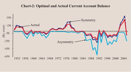
The correlation coefficient of 0.78 between the actual and optimum current account is much lower than symmetry model while the variance ratio of 1.99 is higher than the corresponding symmetry model. The actual and the estimated optimal current from symmetry and asymmetry models are shown in chart 2. It can be seen that the estimates from symmetry model tracks the optimum more accurately than the asymmetry model and the latter is consistently biased towards deficit. Furthermore, the gap between them gets larger from the beginning of the 1990s, expectedly reflecting inappropriateness of asymmetry model in the more liberalized regime on capital flows witnessed since then.10
 Thus, there is only a weak evidence of asymmetry in international capital flows to India. The extent of capital flows had been high enough to allow the private sector to smooth out their consumption path to a large extent. But, this behaviour is primarily attributable to the development during the post-reform period, where correction as well as a greater freedom on capital flows through liberalisation has taken place. However, the optimal current account balance has been larger than the actual current account balance. This is intuitively appealing as there was severe foreign exchange restrictions in the pre-reform period which restricted the smoothing of private consumption up to the optimal level.
Section III
Concluding Observations
Based on constructed time series data on private consumption for the period 1950-51 to 2005-06, we analyse the behavior of India’s current account balance from the following standpoints. First, is the current account balance in India solvent, and if so, can it be attributed to the post-reform period? Second, are the controls on capital flows in India effective and whether there is asymmetry in the controls on capital inflows and outflows? Consequently, is the volatility of capital flows between India and the rest of the world consistent with the expected changes in fundamentals?
We find that inter-temporal model of current account balance is consistent with Indian data. The current account balance, which was inter-temporally insolvent during the pre-reform period, has turned solvent during the post-reform period. This is primarily a reflection of the developments that have taken place during the post-reform period, when restrictions on capital flows have been significantly liberalised. In other words, till the payment crisis of 1990-91, private consumption in India was not optimal and did not reflect the future change in national cash flows. This has changed with the corrections carried out since reforms and the change in current account balance reflects smoothing of private consumption.
We do find some evidence of asymmetry between capital flows, which is on expected lines as restrictions on capital outflows from India have been more than those on inflows to India. The extent of capital flows had been high enough to allow the private sector to smooth out their consumption path to a large extent. But, this behavior is primarily attributable to the development during the post-reform period, where correction as well as a greater freedom on capital flows through liberalisation has taken place. However, the optimal current account balance has been larger than the actual current account balance. This is intuitively appealing as there were severe foreign exchange restrictions in the pre-reform period which restricted the smoothing of private consumption up to the optimal level.
The policy with respect to the gradual opening of the capital account is consistent with the presumption of enabling the agents to smooth consumption to desired optimal level. With further liberalisation of capital flows, both inflows and outflows, it would be possible for agents to further smoothen their consumption to desired optimal level, allowing scope for higher current account deficit to attain potentially higher growth.
Notes:
1 This is referred to as test for orthogonal restrictions.
2 External shocks were in the form of war, oil price hikes and sudden reversal of remittances flows. Even in the worst year of 1991 the deficit to GDP was 3.1 per cent only, much lower than the often-prescribed threshold of 5.0 per cent of GDP. Milesi-Ferretti and Razin (1996), however, notes that a specific threshold level in itself is not sufficiently informative on sustainability and an impending crisis, and needs to be seen in conjunction with the exchange rate policy and structural factors such as degree of openness, levels of savings and investment, and the health of the financial system.
3 Theoretically, by national income identity, the current account balance derived as gross national product less investment less government consumption expenditure less private consumption expenditure should be the same as saving minus investment.
4 It may be noted that earlier studies on India viz., that Ghosh and Ostry (1995) and Callen and Cashin (1999) do not convert the series to a per capita basis, as done by us here.
5 The various selection criterions on the order of VA R show that the appropriate order of VAR is one.
10 As presence of asymmetry is weak, the model performance is thus adversely affected with decomposition of data.
References:
Agenor, Pierre-Richard, Claude Bismut, Paul Cashin and C. John McDermott (1999), “Consumption Smoothing and the Current Account: Evidence for France, 1970-96,” Journal of International Money and Finance, 18, 1-12.
Callen Tim and Paul Cashin (1999), “Assessing External Sustainability in India,” IMF Working Paper, WP/99/181, December.
Cashin, Paul and C. John McDermott (1998a), “Are Australia’s Current Account Deficits Excessive,” The Economic Record, 74(227), December, 346-361.
Cashin, Paul and C. John McDermott (1998b), “International Capital Flows and National Creditworthiness: Do the Fundamental Things Apply as Time Goes By,” IMF Working Paper, WP/98/172, December.
Frenkel, J. and A. Razin (1987), Fiscal Policies and the World Economy, MIT Press, Cambridge, Massachusetts.
Ghosh, Atish R. (1995), “International Capital Mobility Amongst the Major Industrialised Countries: Too Little or Too Much,” The Economic Journal, 105, 107-128.
Ghosh, Atish R. and Jonathan D. Ostry (1995), “The Current Account in Developing Countries: A Perspective from the Consumption-Smoothing Approach,” The World Bank Economic Review, 9, No.2.
Guest, Ross S. and Ian M. McDonald (1998), “The Socially Optimal Level of Saving in Australia, 1960-61 to 1994-95,” Australian Economic Papers, 37(3), September, 213-235.
Hakio, Craig S. and Mark Rush (1991), “Is the Budget Deficit ‘Too Large’,” Economic Inquiry, 29, 429-45.
Hansen, B. (1991), “Testing for Parameter Instability in Linear Models,” Journal of Policy Modeling, 14(4), 517-533.
Kim Kunhong, Viv B. Hall and Robert A. Buckle (2002), “New Zealand’s Current Account Deficit: Analysis Based on Intertemporal Optimisation Approach,” Treasury Working Paper, 01/02.
Milbourne, Ross and Glenn Otto (1992), “Consumption Smoothing and the Current Account,” Australian Economic Papers, 31, December, 369-384.
Milesi-Ferretti, G. Maria and A. Razin (1996), Current Account Sustainability, Princeton Studies in International Finance No. 81, October 1996, Princeton University, Princeton, New Jersey.
Nason, James M. and John H. Rogers (2003), “The Present-Value Model of the Current Account Has Been Rejected: Round Up the Usual Suspects,” International Finance Discussion Papers, No. 760, February, Board of the Federal Reserve System, Canada.
Obstfeld, M. and K. Rogoff (1996), Foundations of International Macroeconomic, MIT Press,
Cambridge, Massachusetts.
Otto Glenn (1992), “Testing a Present-Value Model of the Current Account: Evidence from US and Canadian Time Series,” Journal of International Money and Finance, 11, 414-430.
Otto, Glenn (2003), “Can an Inter-temporal Model Explain Australia’s Current Account Deficit,” School of Economics UNSW Sydney 2052, February. |