India witnessed differential regional impact of the COVID-19 pandemic on economic activity. We construct an economic activity index at regional level to understand the drivers of asymmetry in economic impact and subsequent recovery trajectories. We find that differences in economic structure played a key role. States with higher share of agriculture and mining in their Gross State Value Added (GSVA) witnessed a lower contraction in economic activity vis-à-vis States with higher share of industry and services, necessitating differential policy responses in States supplementing national policy response to mitigate the impact of the pandemic. Introduction The Indian economy is composed of heterogenous regional units which have different economic trajectories. It is critical for policy makers to take cognisance of the regional and spatial dimensions of economic activity for effective policy making and implementation. The overall economic development of a country is crucially dependent on the equitable progress of its States/regions. To this end, economic monitoring of the regions and sub-national units becomes important. Currently, overall economic activity at the State level can be measured by Gross State Domestic Product (GSDP) data which is available annually. As evident during the pandemic, near real time monitoring of the economic activity at State level is important for quick policy responses calibrated to regional conditions. High frequency indicators available at State level provide a sectoral instead of an overall economic picture of the State. In this context, an index capturing the aggregate economic scenario at the regional level is imperative. During the COVID-19 pandemic, lockdowns created disruptions in economic activity, supply chains, nature of work and migration patterns. With the Union Government giving a broad direction and policy support, States and local governments took the lead in adapting and implementing policies according to their specific local conditions. As a result, economic recovery is expected to vary across States. In this context, we construct an economic activity index to measure the diverse economic trajectories across States. The economic structure of the regions may be one possible explanation for the asymmetric economic impact induced by COVID-19 lockdowns and mobility restrictions. The rest of the paper is organised as follows: Section II provides a review of the literature on regional economic activity indices across the world, as well as the literature specific to India. Section III briefly describes the data and Principal Component Analysis (PCA) methodology used for constructing the regional economic activity index. Section IV presents the index at State level. Section V discusses the relationship between economic structure and impact on economic activity and Section VI concludes the article. II. Literature Review The need for a real time measurement of economic performance has been recognised by policy makers across the world. Globally, there are several indices to measure economic activity at a sub-national level. The Federal Reserve Bank of Philadelphia produces a monthly coincident index for each of the 50 States. A dynamic single-factor model is used to create the State indexes using four variables viz., non-farm payroll employment, average hours worked in manufacturing by production workers, the unemployment rate, and wage and salary disbursements. Texas Leading Index by Dallas FED is used to predict economic activity in the State. It uses eight leading indicators viz., Texas value of the dollar, U.S. leading index, real oil price, well permits, initial claims for unemployment insurance, Texas stock index, help-wanted index and average weekly hours worked in manufacturing to arrive at a composite index. Habli et al. (2020) proposed four experimental composite economic activity indices in the context of Canada using PCA and a mix of other methods. The Reserve Bank of New Zealand has developed experimental Regional Activity Index (RAI) to track how regional economies are performing in near real-time. Each regional index summarises 6 monthly indicators of economic activity, covering consumer spending, jobseeker numbers, online job vacancies, traffic volumes (light and heavy vehicles), and electricity demand. Reserve Bank of New Zealand uses PCA methodology to arrive at the weights used to calculate the index. The Chicago Fed National Activity Index (CFNAI) is a weighted average of 85 monthly indicators of national economic activity. It was found that a single index constructed from the first principal component of 85 economic activity series could forecast inflation effectively. The economic indicators used for the CFNAI are drawn from four broad categories of data: i) production and income; ii) employment, unemployment, and hours; iii) personal consumption and housing; and iv) sales, orders, and inventories. Indexes such as the CFNAI provide useful information on the current and future course of economic activity and inflation in the United States. In India, Bhadury et al. (2020) constructed single-index dynamic factors using 6, 9 and 12 high-frequency indicators at the national level. Kumar (2020) constructed an economic activity index for India from 27 monthly indicators using a dynamic factor model. The study uses monthly indicators representing industry, services, global and miscellaneous activities to gauge the underlying State of the economy. However, such research at sub-national or regional level are relatively scarce in the Indian context. In this backdrop, we attempt to construct a composite index of economic activity at regional level for the Indian sub-national units. The index is a composite of six high frequency monthly indicators reflecting the economic activity at a regional level using PCA method. III. Variables and Composite Data Analysis Variable selection is the most crucial part of the exercise to construct an economic activity index at the State-level. Our aim is to include indicators that capture the pronounced and persistent movements in economic activity. To capture the trend of economic activity across States on a monthly basis, a composite index using PCA technique is constructed for the select 18 States1. These States were taken based on coherency of data availability and to avoid missing values for the selected time period. The variables considered in this paper are: i) Goods and Services Tax (GST) collections; ii) electricity generation; iii) employment rate; iv) exports; v) Mahatma Gandhi National Rural Employment Guarantee Scheme (MGNREGS) work demand and vi) Deposits in accounts under Pradhan Mantri Jan Dhan Yojana (PMJDY). These indicators represent activities covering multiple sectors in the economy. The data ranges from March 2020 to February 2022. Since rise in GST collections reflects a rise in economic activity, it is taken as one of the crucial indicators of economic activity at State level. Electricity generation can be construed as an indicator of performance of industrial sector in the economy, thereby being an important reflector of economic activity. Employment rate is another indicator which has a direct bearing on output and income. Higher employment rate augurs well for higher economic growth and vice-versa. Another important variable is exports which is a part of overall output produced in the State. Rise in exports would mainly be the result of higher output production and thus reflect higher economic activity. The MGNREGS work demand is considered as a vital indicator for the rural economy. Increase in work demand under MGNREGS may reflect downturn in economic activity at rural level because demand for MGNREGS work increases when people do not find alternate livelihood opportunities in the event of a slump. This trend was particularly evident during the COVID-19 induced slowdown in the economy, thereby indicating the significance of this variable in gauging economic activity at State level. Deposits under PMJDY accounts mainly belong to informal and unorganised sector workers. Rise in the deposits under PMJDY accounts may reflect a rise in income of the informal workers and thus indicate an uptick in economic activity. A composite indicator is used to represent multiple dimensions of economic activity to arrive at a single indicator. This indicator is used to analyse various dynamics of economic activity. A multivariate analysis is used to study the overall structure of the dataset, assess its suitability, and guide subsequent methodological choices (e.g., weighting, aggregation). III.1: Principal Component Analysis (PCA) Researchers generally use a set of data analysis techniques. For instance, Cronbach Coefficient Alpha technique (henceforth, C-alpha) (Cronbach, 1951) is the most common estimate of internal consistency of items in a model or survey. However, the weakness of C-alpha technique is that correlations do not necessarily represent the real influence of the individual indicators on the phenomenon expressed by the composite indicator. Cluster Analysis (CLA) technique, which will always produce a grouping, is a purely descriptive tool and may not be transparent if the methodological choices made during the analysis are not clearly explained. Canonical Correlation Analysis (CCA) is another technique which can be used to investigate the relationship between two groups of variables. In CCA, a way to classify variables (or cases) into the values of a dichotomous dependent variable is given by Discriminant Function Analysis (DFA). However, DFA is based on several assumptions, like low correlation of the predictors, linearity and additivity, and adequate sample size which limits its use (OECD, 2008). There are challenges in assessing the underlying performance of Indian States using high frequency indicators and empirical exercise. For instance, the choice of appropriate indicators from a large set of potential indicators and with a single extraction from the chosen indicators, may reflect short-term idiosyncrasy rather than an underlying general trend. In the absence of monthly data for GSVA for the given period, it is difficult to use other empirical tools. We use PCA method to develop a composite indicator that can trace the turning points and trends in activity indicators. This article describes the process to derive an economic activity index to mimic trends in aggregate output data at State-level by performing PCA on various characteristic representative variables. The main advantage of this method over the traditional methods is that it avoids many of the measurement problems associated with other methods, such as recall bias, seasonality, and data collection time. Compared with other statistical alternatives, PCA is computationally easier, and uses all of the variables in reducing the dimensionality of the data. PCA converts high-dimensional data to low-dimensional data. Moreover, it improves algorithm performance by removing correlated features along with minimising information loss. III.2 PCA Methodology The PCA works by extracting the maximum variance (largest eigenvalue) across different dimensions of the data set. In this context, we construct monthly economic activity index from different high-frequency variables. Our selection of high-frequency variables is based on criteria such as: i) State-wise economic indicators represent key sectors of the economy; and ii) the variables are released in a timely manner and without significant publication lag. PCA works by transforming a large set of variables into a smaller one that still contains most of the information in the larger set. Principal components are new variables that are constructed as linear combinations of the initial variables that try to capture most of the information from the original set of variables. In mathematical terms, from an initial set of n correlated variables, PCA creates uncorrelated indices or orthogonal components, where each component is a linear weighted combination of the initial variables. For example, from a set of variables X1 to Xn, principal components are where amn represents the weight for the mth principal component and the nth variable. In order to overcome the potential bias in index generated due to large differences between the range of various variables, it is vital to perform standardization of all the variables prior to applying PCA technique. Subsequently, covariance matrix is constructed from which, eigenvectors and eigenvalues will be derived which is key to compute principal components to construct an index. The covariance matrix is a n × n symmetric matrix that has entries as the covariances associated with all possible pairs of the initial variables. For example, for a 3-dimensional data set with 3 variables x, y, and z, the covariance matrix is a 3×3 matrix of this form: In order to determine the principal components of the data, eigenvectors and eigenvalues are computed from the covariance matrix. Every eigenvector has an eigenvalue and their number is equal to the number of dimensions of the data. The variance (λi) for each principal component is given by the eigenvalue of the corresponding eigenvector. By ranking eigenvectors in order of their eigenvalues, highest to lowest, we get the principal components in order of significance. Subject to the constraint that the sum of squared weights is one, the components are ordered in descending order based on amount of variation explained by them in data set. The first component (PC1) explains the largest possible amount of variation in the dataset. The proportion of the total variation in the original data set accounted by each principal component is given by λi /n, because the sum of the eigenvalues equals the number of variables in the initial data set (Vyas & Kumaranayake, 2006). Subject to the same constraint, the second component (PC2) is completely uncorrelated with the first component. The second component explains less variation than the first component. However, each component captures an additional dimension in the data because subsequent components are uncorrelated with previous components; but explains smaller and smaller proportion of the variation in the original data set. I n the present study, we have considered first principal component to construct the index. A standardised value of the level of the variables in the PCA is calculated. A positive value of the index means that the activity was above average and vice-versa for a negative value. The index should be used as indicator of regional economic momentum. For example, if a given index value increases (decreases) over the course of several consecutive months for any particular State, that can be taken as a signal that conditions in the regional economy are improving (worsening). Similarly, several consecutive months of positive values can be taken as a signal that activity in that region is rising at above-average level and vice-versa. IV. Economic Activity Index at State level The COVID-19 pandemic and consequent lockdown led to a severe downfall in economic activity across the States (Table 1). This is reflected in a sharp dip in index value across the States in the months of April and May 2020. Consequently, as the severity of pandemic started reducing across the States, relative improvement in the index value is evident in the ensuing months. However, with the arrival of second wave, economic activity was hampered again, though less severely than the first pandemic wave. This was reflected in the relatively lower contraction of the index in the States compared to the first wave. Subsequently, with focus on rapid vaccination and better preparedness on health front among other steps, the effect of Omicron wave was less severe on both lives and livelihood. The index remained positive in December 2021 and January 2022 across the States despite the Omicron wave. During the month of April 2020, as the economic activity was undergoing an overall fall across the States, relatively higher impact was seen in Rajasthan and Maharashtra. During the second wave induced economic shock, States like Odisha, Jharkhand and Chhattisgarh witnessed a lower decline in economic activity. While Telangana, Assam and West Bengal saw a relatively higher impact on economic activity. Subsequently, as the Omicron variant hit the country, many States’ economies were able to withstand its impact as can be inferred from the positive values of the index across the States. Thus, there was a distinct spatial pattern for the impact of COVID-19 on economic activity in Indian States. Lockdown induced mobility restrictions impacted States in different ways. In the following section, this article shows that one possible explanation for this distinct economic impact could be the varied economic structure of these States. V. Empirical Analysis As a result of social distancing and lockdown during COVID-19, daily mobility and lifestyle-related habits have changed in a significant manner. IMF (2021) quantifies the impact of containment measures and voluntary social distancing on both the spread of the virus and the economy at the State level during the first wave of the COVID-19 pandemic. State-level empirical analysis suggests that social distancing and containment measures effectively reduced case numbers but came with high economic costs. Beyer et al. (2021) used daily electricity consumption and monthly night-time light intensity data to measure economic activity in India. They show that not all States and Union Territories have been affected equally. Part of the heterogeneity is explained by the prevalence of COVID-19 infections, the share of manufacturing, and return migration. Meinen et al. (2021) conduct ex-post analysis of the determinants of within-country regional heterogeneity of the labour market impact of COVID-19. The study finds that the propagation of the economic impact across regions cannot be explained by the spread of infections only. Instead, a region’s economic structure is a significant driver of the observed heterogeneity. In this context, we analyse a pertinent question; how the impact of COVID-19 manifest at the State level taking into account differences in economic structure of various States. The impact of lockdowns was evident on economic activity during the pandemic. Various policy measures taken by the governments across the States to contain the spread of the virus reduced the mobility of people. The strictness of the mobility restriction measures, and its implementation is reflected in the google mobility data (Table 2). This data is used as a proxy to reflect the stringency of the lockdown measures. Higher mobility restrictions were clearly associated with the fall in economic activity index during the first wave of the pandemic. The months of April and May 2020 had the most stringent lockdown and the economic activity also witnessed sharp contraction in these months. During the second wave, mobility restrictions were relatively milder leading to a less severe impact on economic activity. Moreover, as the Omicron wave hit the country, the lockdowns were only marginal as a result of which economic activity continued to steer on a positive trajectory. Lockdown had a direct impact on economic activity necessitating it to be used in a calibrated and well-thought-out manner and to be used as a last resort so that economic activity can be restored swiftly through suitable measures.  However, there is relatively differential impact of the mobility restrictions on the economic activity across the States. It was found that prolonged mobility restrictions in some States had higher debilitating impact on economic activity. In contrast, some States witnessed a resurgence in economic activity relatively sooner even when they had continued mobility restrictions for longer periods. The restrictions on mobility impacted economic activity across the States with varying intensity (Chart 1). The varied economic structure and sectoral composition of the States was one possible reason for differential impact on economic activity (Chart 2). The States that were dependent more on agriculture and allied activities coupled with mining and quarrying were observed to have relatively better economic scenario amidst the pandemic. Agriculture sector continued to be the silver lining witnessing the least decline in growth. Within Services sector, some services witnessed a benign impact due to the work from home/work from anywhere policy of the companies and robust use of internet for seamless continuation of work. However, contact intensive services were the most negatively impacted, while services like public administration tried to provide a cushion against significant downfall in services. States having economic structure with dominance of manufacturing, also, witnessed the brunt of lockdown more than others. 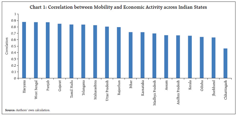
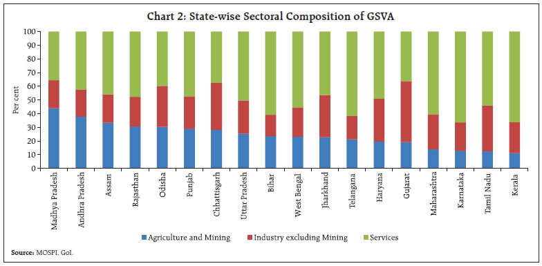 The charts presented in the subsequent section show the relation between economic structure of the State and impact of mobility restrictions on overall economic activity. The downward sloping nature of the curve would mean that States with higher share of the mentioned sub-sector in GSVA (the value on the Y axis is greater) have low correlation between economic activity and mobility (the value on the X axis is lower) thereby leading to lower impact of mobility restrictions on overall economic activity of the State. This means States which had higher share of that sector were relatively less impacted due to mobility restrictions vis-à-vis other States. In other words, downward sloping curve means that mobility restrictions had relatively lower impact on the overall economic activity thereby indicating that higher share of that sector in GSVA strengthened State’s economic resilience against lockdown induced mobility restrictions in comparison to other States. V.1 Agriculture The correlation between mobility and economic activity index was found to be lower for States which have higher share of agriculture in their GSVA (Chart 3a). This indicates that States with relatively greater share of agriculture have witnessed a lower impact on economic activity. Agriculture sector has proved to be resilient amidst the COVID-19 induced economic shock. Within agriculture sector, States which are more dependent on forestry and logging witnessed a relatively lower impact on economic activity as reflected in the lower correlation between mobility and economic activity for States with high share in forestry and logging (Chart 3b). V.2 Industry The Industrial sector was severely hit due to supply chain disruptions, shortage of migrant workers due to reverse migration and less demand. States with higher dependence on manufacturing were found to have higher correlation between economic activity and mobility thereby leading to greater impact of mobility restrictions on these States (Chart 4a). With higher share of manufacturing and high correlation between mobility and economic activity, mobility restrictions had a more profound impact on overall economic activity. Within industry sector, however, States with high share of mining and quarrying had a low correlation between mobility and economic activity indicating lower impact of mobility restrictions on economic activity in such States (Chart 4b).
V.3 Services Services sector has been heavily affected by the COVID-19 outbreak. Given the sector’s role in providing inputs for other economic activities, it witnessed a significant economic impact. Within services sector, States with higher share of contact intensive services like trade, hotels, transport, storage and communication were found to have high correlation between mobility and economic activity and vice-versa. This clearly indicates that the mobility restrictions had much higher impact on economic activity in States having more dependence on contact-intensive services (Chart 5a and 5b). VI. Conclusion COVID-19 has left a lasting imprint on the State economies, causing permanent changes. State-wise economic activity index reveals the massive and unprecedented downfall brought by the COVID-19 led disruptions in the State economies. The associated lockdowns and mobility restrictions, however, brought differential impact across the States. The economic structure of respective States has played a significant role in influencing their economic trajectories in the aftermath of COVID-19 induced restrictions. It was found that States with higher share of agriculture and mining in their GSVA witnessed a more resilient economic path vis-à-vis States with higher share of industry and services. Within agriculture sector, States with higher share of forestry and logging in GSVA witnessed a relatively lower impact on economic activity. It was also evident that States with high share of manufacturing and services in their GSVA witnessed relatively more impact on economic activity. Apart from the economic structure, it is, however, possible that the relationship between mobility and economic activity may be influenced by other factors, including varied localised mobility restrictions and adaptive policy responses in different States. Adding these factors will further enrich the analysis, however, such formal analysis requires availability and quantifiability of data, which is scarce at this point in time. Such granular analysis at sub-sectoral level and of economic structure has emphasized the need and importance to have a differential policy response by the States based on their respective economic structure supplementing the national policy interventions. This will ensure that, during such massive crisis, well-informed and coordinated policy decisions at the national and State-level will lead to minimum loss in overall economic activity and wheels of economic development will recover swiftly after major economic disruptions. References Bhadury, S., Ghosh, S., and Kumar, P. (2020), “Nowcasting Indian GDP Growth Using a Dynamic Factor Model”, RBI Working Paper Series No. 03. Beyer, R. C., Franco-Bedoya, S., and Galdo, V. (2021), “Examining the economic impact of COVID-19 in India through daily electricity consumption and nighttime light intensity”, World Development, 140, 105287. Cortina, J. M. (1993), “What is coefficient alpha? An examination of theory and applications”, Journal of applied psychology, 78(1), 98. Crone, T. M., and Clayton-Matthews, A. (2005), “Consistent economic indexes for the 50 states”, Review of Economics and Statistics, 87(4), 593-603. Cronbach L. J. (1951), “Coefficient alpha and the internal structure of tests”, Psychometrika, 16: 297-334. Deb P, Furceri D, David J, and Tawk N (2020), “The Effect of Containment Measures on the COVID-19 Pandemic”, IMF Working Paper, August. Habli N., Macdonald R. and Tweedle J. (2020), “Experimental Economic Activity Indexes for Canadian Provinces and Territories: Experimental Measures Based on Combinations of Monthly Time series”, Analytical Studies Branch Research Paper Series, Statistics Canada. IMF (2020), “The Great Lockdowns”, World Economic Outlook, April. Jobson, J. D. (1992), “Principal components, factors and correspondence analysis”, Applied multivariate data analysis (pp. 345-482), Springer, New York, NY. Joint Research Centre-European Commission. (2008), “Handbook on constructing composite indicators: methodology and user guide”, OECD publishing. Kumar P. (2020), “An Economic Activity Index for India”, RBI Bulletin, November 2020. McLachlan G., (2004), “Discriminant Analysis and Statistical Pattern Recognition”, NY: Wiley-Interscience, Wiley Series in Probability and Statistics. Meinen, P., Serafini, R., and Papagalli, O. (2021). Regional economic impact of Covid-19: the role of sectoral structure and trade linkages. Working Paper Series 2528, European Central Bank. Kishore N., Kahn R. and others (2021), “Lockdowns result in changes in human mobility which may impact the epidemiologic dynamics of SARS-CoV-2”, Scientific Report. (https://www.nature.com/articles/s41598-021-86297-w.pdf) Regional Activity Indices (RAIs), Treasury of New Zealand. https://www.treasury.govt.nz/publications/research-and-commentary/regional-activity-indices. Vyas S., and Kumaranayake L. (2006), “Constructing socio-economic status indices: how to use principal components analysis”, Health policy and planning, 21(6), 459-468.
|