by Deba Prasad Rath, Silu Muduli and Himani Shekhar^{^}

This study integrates the “Inflation at Risk” (IaR) and “Growth at Risk” (GaR) frameworks to identify stagflation risk in India. Elevated risks of stagflation were experienced during specific episodes like the Asian Crisis, the Global Financial Crisis, the taper tantrum, and the COVID-19 pandemic. The empirical findings suggest supply-side shocks such as spikes in commodity prices along with tighter financial conditions and relatively higher depreciation of domestic currency are the major determinants of stagflation risk in India.

Introduction

Post COVID-19 pandemic, the global economic landscape faced challenges that led to an increased risk of stagflation, portmanteau of economic stagnation alongside high inflation. Various factors, such as the COVID-19 pandemic, geopolitical tensions, lockdowns in China, and supply chain disruptions, have contributed to this situation (World Bank, 2022). However, compared to stagflationary period of the 1970s, currently the risk of stagflation is lower attributable to favourable macroeconomic conditions. Unlike the severe commodity price shocks experienced in the 1970s, during which crude oil almost increased four-fold, the increase in energy prices during 2022 was lesser. Additionally, central banks worldwide are now more focused on maintaining price stability and, financial institutions have healthier financial positions. The long-term inflation expectations are well-anchored to the inflation target unlike during the 1970s when inflation expectations were weakly-anchored and went to exorbitantly high levels (Pattanaik et al., 2023). These factors collectively contribute to limiting the risk of stagflation in the current global landscape compared to the 1970s.

Historically, various events during the last two decades including global financial crises, the taper tantrum, and the COVID-19 pandemic have increased risks of stagflation. Recent evidence from 22 economies that rely heavily on non-commodity exports highlights two significant factors that could elevate the risk of stagflation in emerging markets - higher commodity prices and the appreciation of the US dollar (Hofmann et al., 2023). These factors can lead to weak economic growth and high inflation exacerbating the stagflationary risk in these economies. Post COVID-19 pandemic, the delays in the monetary normalisation process have also raised concerns of costly stagflation (Enders et al., 2022) as pursuing price stability along with an accommodative stance by monetary authorities may lead to the de-anchoring of inflation expectations (Dierks, 2023). Such situations might give rise to delicate trade-offs resulting in financial instability as tightening financial conditions in response to such instability can further deepen the economic slowdown (Canuto, 2022).

India as an emerging market economy also faced challenges post-COVID-19 with a pickup in inflation along with weak demand initially raising stagflation risks. Stagflation risk becomes a concern for policymakers as it has the potential to destabilise the entire macroeconomic framework of the economy through creating an environment of uncertainty. The Reserve Bank of India (RBI) is entrusted with the primary objective of maintaining price stability while keeping in mind the objective of growth¹ which requires constant monitoring of any arising stagflation risk. In the Indian context, Ghosh et al. (2023) uses Growth at Risk (GaR) framework for assessing the entire distribution of future GDP growth and quantifying the likelihood of lower quantiles of GDP growth. While for inflation, Muduli and Shekhar (2023) estimate tail risks of consumer price index (CPI) inflation in India using a quantile regression framework. However, none of the studies have analysed the risks to growth and inflation together in the case of India even though these are interconnected macroeconomic issues. These factors motivate us to empirically examine the risk of stagflation in India in the current macroeconomic environment.

This study focuses on identifying risk factors for stagflation, which is characterised by periods of recession coupled with high inflation. It attempts an assessment of the stagflation risks by examining the role of some key variables such as financial conditions, the exchange rate [(INR) against the United States Dollar (USD)] and crude oil price. In a parallel analysis, the study integrates the “IaR” and “GaR” frameworks (Adrian et al., 2019; Banerjee et al., 2020) to redefine stagflationary situations and evaluate risks to it. The empirical findings reveal that tightening financial conditions and exchange rate depreciation significantly contribute to stagflation, while crude oil prices portray a limited impact even though India depends significantly on crude oil imports. The limited impact of crude oil prices to stagflation risk reflects the partial pass-through of global crude oil prices to domestic pump prices which contains the pass-through of input cost pressures to growth as well as inflation. Encouragingly, the estimated results indicate that recent improvements such as eased financial conditions, moderate domestic currency depreciation and stable crude oil prices have helped reduce the risk of stagflation in India.

The study is structured as follows: Section II provides a brief review of the existing literature on stagflation and recent perspectives. In Section III, some stylised facts, data description along with empirical analysis and results are presented. Finally, Section IV presents the conclusions of the study offering insights into the current macroeconomic situation and the potential risk of stagflation.

II. Review of Related Literature

The stagflationary situation experienced in the 1970s was primarily driven by a substantial spike in international crude oil prices. Some researchers argued that it was also impacted adversely by the implementation of a tightening monetary policy aimed at stabilising prices (Bernanke et al., 1997; Jiménez-Rodriguez et al., 2010). However, the effectiveness of this policy in managing supply-side shocks was limited. Barsky et al.(2001) provided insights into the relationship between price fluctuations and economic fluctuations, highlighting that the coincidence of an oil price shock with an economic contraction contributed to the stagflationary situation in the 1970s. Moreover, during that period, uncertainty in monetary policy led to a costly disinflationary process. Since then significant progress has been made in reducing this uncertainty with the widespread adoption of inflation targeting in various advanced and emerging market economies (Khan et al., 2015).

The 1970s episode was further exacerbated by higher import prices and low productivity levels, which deepened the economic downturn (Grubb et al., 1982). A critical aspect that emerged was the rational perception of economic agents regarding persistently high inflation and unemployment. Such a perception can have detrimental effects on overall productivity (Brunner et al., 1980).

In more recent episodes, delays in the monetary normalisation process have raised concerns about the potential for a costly stagflation (Enders et al., 2022). The pursuit of price stability by monetary authorities, if combined with an accommodative stance, can lead to the de-anchoring of inflation expectations, in turn, destabilising inflation dynamics (Dierks, 2023). This creates a delicate trade-off that may also result in a situation of financial instability. Tightening financial conditions in response to such instability can further deepen the economic slowdown (Canuto, 2022).

Literature in the Indian context remains scanty in this field. Muduli and Shekhar (2023) have estimated tail risks of inflation for various macroeconomic situations that include supply-side shocks and their adverse impact on both upper and lower tail risks of inflation in India. Similarly, Growth-at-risk framework for real GDP growth has been used to analyse the low probability extreme events for monitoring risks to financial stability and macro-prudential policy implementation (Ghosh et al., 2023). Nonetheless, to the best of our knowledge we have not come across studies in the Indian context that together estimate the risks to growth and inflation i.e., stagflation risk. This study would try to fill this gap by analysing the risks to stagflation and also integrating both the GaR and IaR.

Given the global economic landscape considerably impacted by various events, such as the COVID-19 pandemic, Ukraine-Russia tension, rising commodity prices, and supply-side disruptions, Siddiqui (2022) highlighted the need for globally coordinated policies to mitigate stagflation risks. In light of these challenges, this study aims to estimate the risk of stagflation in India where periods of recession coupled with high inflation are considered as stagflationary situations by examining key variables such as financial conditions, exchange rate depreciation, and crude oil prices. In order to add robustness to the estimates, the study would incorporate the concepts of GaR and IaR to redefine stagflationary situations (Adrian et al., 2019; Hofmann et al., 2023). This holistic approach will enhance the study’s accuracy in identifying the key determinants of stagflation risk for the Indian economy and contribute to the nascent literature.

III. Empirical Analysis

Stylised Facts

After the COVID-19 pandemic, several factors including pent-up demand for goods and services, supply chain disruptions, rising energy and commodity prices, monetary stimulus, and depreciation of domestic currency caused concerns for the global economy. The initial slump in demand by job losses and lockdowns were soon replaced by pent up demand once restrictions were lifted. There were issues with production, labour availability, supply chains, and availability of raw materials. To boost the economy, both fiscal and monetary stimulus was provided globally. Consequently, gradually demand started recovering faster than the recovery in supplies leading to pick up in commodity prices and domestic currency depreciation. This situation posed a risk of prices going up, leading to higher inflation, while also posing a risk of slower economic growth.

Global commodity prices picked up during the years 2021-22 and 2022-23 post the dip seen in 2020-21 raising concerns for both inflation and economic growth as prices of energy, metals and agricultural inputs rose resulting in input cost pressures (Chart 1.a). Higher commodity prices can lead to increased production costs reducing profit margins potentially discouraging investment and expansion plans. If businesses are unable to absorb the higher costs, they may pass them on to consumers, exacerbating inflationary pressures. Moreover, currency depreciation in 2022-23 by 7.9 per cent raised risks of imported inflation as well as higher imported costs for firms (Chart 1.b). These twin risks from higher global commodity prices and currency depreciation raised concerns of stagflation globally.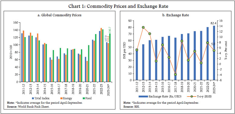

Post pandemic, stagflation issue needed careful attention from the policy makers to support the economy. Supply chain issues arose after the pandemic in response to lockdowns and production delays in different parts of the world particularly during 2021-22 leading to shortage of inputs and containers which raised concerns for growth and inflation (Chart 2.a). A higher value of India Supply Chain Pressures Index (ISPI)² indicates supply chain pressures.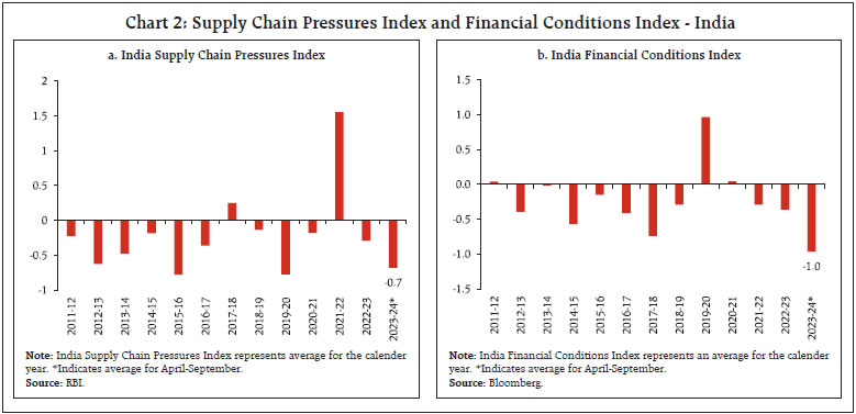

While stagflation is usually a result of supply shocks such as a sudden spike in commodity prices, the risks could also propagate through knock-on effects through their impact on other macroeconomic variables such as a sudden depreciation of the exchange rate or a tightening of financial conditions. Growth and inflation, in such a scenario, could be impacted through multiple channels such as increased borrowing constraints for firms or large exchange rate pass-through effects on domestic prices. When firms face higher borrowing constraints, they may respond by raising their prices (Banerjee et al., 2020). This, in turn, poses an additional risk of higher inflation as well as lower economic growth. In essence, the ripple effects of market volatility and tightened financial conditions can have significant implications for both inflation and overall economic growth i.e., higher inflation and lower growth, over and above the direct impact of the supply shock. The tight financial conditions³ prevailing in the economy during 2019-20 were a source of concern for growth (Chart 2.b). A higher value of Citi Financial Conditions Index (FCI) indicates tight monetary conditions, a lower value indicated easy financial condition. However, both supply chain pressures and the tightness in the financial conditions have shown signs of improvement recently suggesting that the situation may be gradually improving.

The sharp pick-up in domestic energy prices since May 2020 posed risks to both inflation and growth outlook as it adds to the cost of production. Besides fuel and light group in CPI, transport subgroup containing petrol, diesel and fares are also impacted by the movement in petroleum products. India being the 3rd largest consumer of crude oil and depending on imports to the tune of around 80 per cent makes the role of supply management very critical for country’s energy security. Prices of petroleum products are mostly administered in the sense OMCs (Oil Marketing Companies) usually announce the prices of LPG, kerosene, petrol and diesel by taking into account base price, dealer’s margin and different duties set by the government. Reflecting all these factors, the pass-through of global crude oil prices to domestic pump prices of petrol and diesel has not always been uniform⁴ (Chart 3) and the correlations between the global crude oil prices and domestic retail prices of petrol and diesel weakened during certain periods (for details please refer to annex Chart A1). This highlights the fact that different factors can have different impacts on the growth and inflation trajectory depending on the underlying dynamics of pass-through.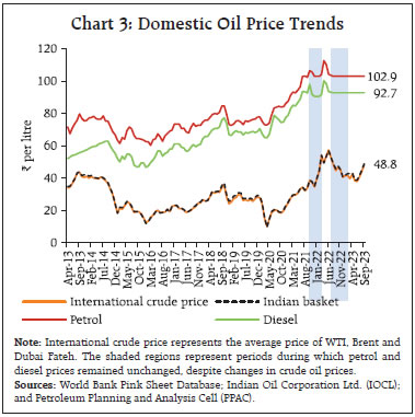

Against this backdrop, we have analysed the past data and observed different phases of inflation and recession in history. Data over the past two decades indicates that India experienced a higher risk of stagflation during global financial crises, the taper tantrum, and the COVID-19 pandemic (Chart 4). India witnessed an economic slowdown in several phases; however, it witnessed inflationary pressures for a prolonged period during the Global Financial Crisis (2007-08). A tight domestic monetary policy and sluggish global growth might have led to the economic slowdown in 2011. The uncertainty and capital outflows resulting from the taper tantrum in 2013 also impacted India’s economic growth momentum. CPI inflation was above 10 per cent in a few months which together with weak growth led to a stagflationary situation. The emergence of the COVID-19 pandemic and elevated inflation in 2020, although for a short period, raised the risk of stagflation.

Data and Methodology

In our empirical analysis, we have utilised quarterly data spanning from Q1:1996-97 to Q2:2023-24 for various indicators to assess and estimate the risk of stagflation. We have taken quarterly real GDP growth provided by the National Statistical Office (NSO). For inflation, CPI headline from 2011 onwards has been considered. While prior to 2011 CPI headline is not available. So, we have used CPI for industrial workers (CPI IW) as a proxy for CPI headline inflation between June 1996 and December 2011. Financial conditions have been incorporated in the estimation by using the Citi India FCI⁵ sourced from Bloomberg. This index helps us understand the overall state of the financial markets and their potential impact on the economy. A higher value of Citi India FCI indicates tighter financial conditions, while a lower value suggests an easing of financial conditions which consequently has an impact on investment decisions as well as costs. For evaluating the credit conditions of the Indian economy, we have relied on the credit-to-GDP ratio, a measure published by the Bank for International Settlements (BIS). This ratio serves as a proxy for understanding the availability and accessibility of credit in the economy. Additionally, we have taken into account the exchange rate dynamics by considering the INR/USD exchange rate published by the RBI as fluctuations in the exchange rate can have significant implications for the economy. Depreciation of domestic currency can potentially lead to imported input costs and imported inflation. Since, energy is an important factor of production and it has a significant weight in the CPI basket, we have incorporated the Indian Basket Crude Oil price in our estimation framework. We propose two approaches to identify the stagflationary phase and examine its determinants. These two approaches are discussed as follows.

Baseline Approach

First, we define a stagflationary situation. At time t, it is said to be a stagflationary situation if it is a recessionary phase and inflation is above the 75th quantile of the historical distribution of inflation

To identify the recessionary phase, we use the methodology proposed by Harding and Pagan (2006) algorithm. First, it detrends the time series data by eliminating the underlying trend component by fitting a polynomial curve to the data and subsequently subtracting this polynomial from the original dataset. Subsequently, the algorithm proceeds to identify turning points within the data. A turning point is recognised when the smoothed data changes direction, specifically when it shifts from being positive to negative. This signifies the presence of a peak in the data. Conversely, a turning point is also identified when the smoothed data transitions from negative to positive, indicating the presence of a trough. Based on this definition, we create a binary dummy variable, which we will refer to as “Stagflation Dummy”. This variable takes a value of 1 if the economy is in a stagflationary phase, indicating both high inflation and stagnant economic growth, and 0 otherwise. To understand the factors contributing to the likelihood of stagflation in India, we investigate the role of three key variables: the Citi India FCI, the INR/USD exchange rate, and crude oil prices. The India Basket crude oil prices has been used as a representative of commodity price shocks. The empirical exercise employs the Probit methodology which uses the above-mentioned explanatory variables to determine the probability of a stagflationary situation. Formally,

Where Y is the dichotomous variable representing the stagflationary situation, X is the set of explanatory variables that includes Citi India FCI, INR/USD exchange rate and India basket crude oil price. Ø is the cumulative standard normal distribution function. The exchange rate explains the defined stagflationary phase in both specifications 2 and 3. Financial conditions also serve as a significant indicator in specification 1. However, the risk from a spike in crude prices is limited and does not turn out to be statistically significant given the weak pass-through of global crude oil prices to domestic petrol and diesel prices.

Integration of Inflation at Risk and Growth at Risk Approach

In order to add robustness to our estimates, we employ another approach where stagflationary situations have been identified by employing the IaR and GaR methodologies. These frameworks allow us to estimate the risk of stagflation both in historical contexts and in the current economic landscape. The “at risk” framework utilises quantile regression to estimate tail risks for inflation and growth, providing insights into potential extreme scenarios identified by the given level of probability parameter (Adrian et al., 2019; Banerjee et al., 2020).

In the IaR framework, we consider various risk factors to assess the likelihood of stagflation. These factors include the output gap, crude oil prices and the INR/USD exchange rate. The output gap provides a measure of the difference between actual and potential GDP, offering insights into an economy’s utilisation of resources. Fluctuations in crude oil prices can lead to a pick up in input costs as well as fuel prices which can impact inflation trajectory. Additionally, the exchange rate (INR/USD) can influence the cost of imports contributing to inflationary pressures.

On the other hand, the GaR framework considers a broader set of indicators to estimate growth risk. These indicators include leading economic indicators from CEIC, financial conditions, credit-to-GDP ratio, and US real GDP growth. Leading economic indicators provide crucial insights into the future direction of economic activity, helping gauge potential risks to economic growth. Financial conditions encompass various aspects of the financial system such as interest rates and credit availability which can impact investment and consumption influencing economic growth. The credit-to-GDP ratio serves as a measure of credit conditions in the economy reflecting the availability of credit and potential risks of financial instability. Finally, considering the US real GDP growth allows us to account for external factors that may affect India’s economic growth given its integration into the global economy.

Using quantile regression, we can estimate tail risks which provide information on extreme outcomes with a given level of probability. Formally, the quantile regression approach is given by:

Where y is the dependent variable which isinflation for IaR and real GDP growth for GaR. X_t is the set of respective explanatory variables as explainedabove for IaR and GaR. The parameter q Ɛ (0,1) is thequantile or probability parameter that is aimed forestimation. This approach allows us to better assessthe potential severity of stagflationary episodes anddevise appropriate policy responses. The IaR forq = 95 per cent and GaR for q = 5 per cent is plottedin Chart 5.

In this scenario, we define a stagflation dummy as a binary variable which takes value 1 when IaR is at the 95th percentile (indicating upside risk to inflation) in the fourth quartile and GaR is at the 5th percentile (indicating downside risk to growth) in the first quartile and, 0 otherwise.

We continue to utilise the probit model defined in equation (1) to estimate the risk of stagflation. This model incorporates factors such as financial conditions, crude oil prices and the INR/USD exchange rate. Tighter financial conditions and depreciation of the exchange rate are found to increase the risk of stagflation whereas crude oil prices have a limited impact on stagflation risk in line with the contained impact of global prices to domestic prices (Table 2).

Our historical analysis reveals specific periods with higher stagflation risk, notably during events like the Asian Crisis (1997-98), the Global Financial Crisis (2007-09), the Taper Tantrum (2013), and the COVID-19 pandemic (Chart 6)⁶. During these identified periods, the risk of stagflation was elevated due to various economic challenges and external shocks. However, the stagflation risk arising post COVID-19 has subsided reflecting easing of financial conditions, contained depreciation of the INR/USD exchange rate and stable domestic petrol and diesel prices. Furthermore, post-pandemic gradual recovery in demand conditions and moderation in CPI headline inflation have been in line of our assessment of reduction in stagflation risk to about 1 per cent (Chart 6).

IV. Conclusion

Stagflation has the potential to destabilise the entire macroeconomic framework of an economy by creating an environment of uncertainty. It is a major concern for the RBI as it is entrusted with the primary objective of maintaining price stability while keeping in mind the objective of growth requiring constant monitoring of any arising stagflation risk. Further, higher commodity prices and the appreciation of the US dollar post-pandemic raised concerns of stagflation globally. The delays in the monetary normalization process after the pandemic have also raised concerns about the potential for a costly stagflation. Against this backdrop, this article attempts to assess the stagflation risk in India and identifies two significant risk factors: financial conditions and depreciation of the INR against the USD. These factors prominently influence the likelihood of stagflation as corroborated by the empirical estimates. Similar results after using the integrated IaR and GaR frameworks to evaluate the stagflation risks adds further credence to our findings. However, given the weak pass-through of crude oil prices to domestic petrol and diesel prices, it has limited predictive power for stagflation.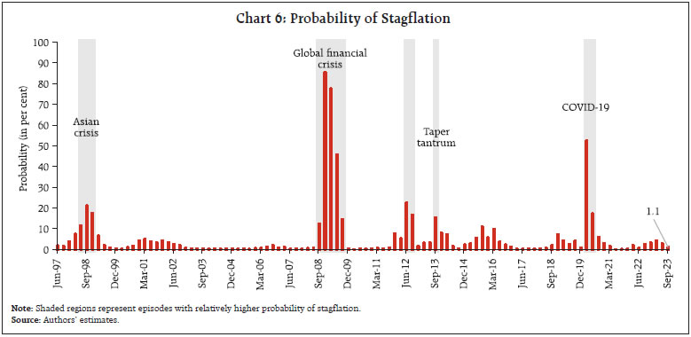

Compared to the historical episodes stagflation risk is currently lower at about 1 per cent which could be attributable to several factors. Commodity price shocks are not as severe and persistent as they were back then. Moreover, given the focus of central banks on maintaining price stability worldwide and healthier financial positions of financial institutions, the long-term inflation expectations have largely remained well-anchored to the inflation target unlike during the 1970s when inflation expectations were weakly-anchored and went to exorbitantly high levels.

References

Adrian, T., Boyarchenko, N., & Giannone, D. (2019). Vulnerable growth. American Economic Review, 109(4), 1263–1289.

Banerjee, R. N., Contreras, J., Mehrotra, A., and Zampolli, F. (2020). Inflation at risk in advanced and emerging economies. BIS Working Papers No. 883

Barsky, R. B., & Kilian, L. (2001). Do we really know that oil caused the great stagflation? A monetary alternative. NBER Macroeconomics Annual, 16, 137–183.

Bernanke, B. S., Gertler, M., Watson, M., Sims, C. A., & Friedman, B. M. (1997). Systematic Monetary Policy and the Effects of Oil Price Shocks. Brookings Papers on Economic Activity, 1997(1), 91.

Brunner, K., Cukierman, A., & Meltzer, A. H. (1980). Stagflation, persistent unemployment and the permanence of economic shocks. Journal of Monetary Economics, 6(4), 467–492.

Canuto, O. (2022). War in Ukraine and risks of stagflation. Policy Center for the New South.

Dierks, L. H. (2023). Monetary Policy and Stagflation: A trade-off between price stability and economic growth? Journal of New Finance, 2(3), 2.

Enders, A., Giesen, S., & Quint, D. (2022). Stagflation in the 1970s: lessons for the current situation. SUERF Vienna.

Ghosh, S., Kamate, V., & Sonpatki, R. (2023). Application of Growth-at-Risk (GaR) Framework for Indian GDP. RBI Bulletin, 78(3), 101–113.

Grubb, D., Jackman, R., & Layard, R. (1982). Causes of the current stagflation. The Review of Economic Studies, 49(5), 707–730.

Harding, D., & Pagan, A. (2006). Synchronization of cycles. Journal of Econometrics, 132(1), 59–79.

Hatzius, J., Hooper, P., Mishkin, F. S., Schoenholtz, K. L., & Watson, M. W. (2010). Financial conditions indexes: A fresh look after the financial crisis.

Hofmann, B., Park, T., & Tejada, A. P. (2023). Commodity prices, the dollar and stagflation risk. BIS Quarterly Review, 33–45.

Jiménez-Rodriguez, R., & Sánchez, M. (2010). Oil-induced stagflation: a comparison across major G7 economies and shock episodes. Applied Economics Letters, 17(15), 1537–1541.

Khan, S., & Knotek II, E. S. (2015). Drifting inflation targets and monetary stagflation. Journal of Economic Dynamics and Control, 52, 39–54.

Mandrekar, J. N. (2010). Receiver operating characteristic curve in diagnostic test assessment. Journal of Thoracic Oncology, 5(9), 1315–1316.

Muduli, S., & Shekhar, H. (2023). Tail Risks of Inflation in India. Reserve Bank of India Working Paper Series No. 2.

Pattanaik, S., Nadhanael, G. V., and Muduli, S. (2023). Taming Inflation by Anchoring Inflation Expectations. Economic and Political Weekly, 58(22), 33-41.

Patra, M. D., Behera, H., and Gajbhiye, D. (2022). Measuring Supply Chain Pressures on India. RBI Bulletin, 77(4), 169–184.

Siddiqui, K. (2022). Problems of Inflation, War in Ukraine, and the Risk of Stagflation. European Financial Review, April/May, 5–13.

World Bank. (2022). Global Economic Prospects Report June 2022. World Bank.

Annex

^{^} The authors are from the Department of Economic and Policy Research (DEPR), Reserve Bank of India, Mumbai. We thank Dr. G V Nadhanael for providing valuable comments. The views expressed are those of the authors and do not necessarily represent the views of the Reserve Bank of India.

¹ Under the Reserve Bank of India, Act,1934 (RBI Act,1934) (as amended in 2016), RBI is entrusted with the responsibility of conducting monetary policy in India with the primary objective of maintaining price stability while keeping in mind the objective of growth.

² ISPI has been developed by extracting common factors latent in domestic and global variables and it tracks supply chain pressures on the Indian economy efficiently (Patra et al, 2022).

³ The financial conditions have been measured using Citi FCI which consists of a weighted average of the following variables: corporate spreads, money supply, equity values, mortgage rates, the trade-weighted dollar, and energy prices.

⁴ For instance, during December 2021- March 2022 global prices increased steeply, but domestic prices increased gradually with a lag indicating contained risks from crude oil prices to growth and inflation during the same period. Further, global crude oil prices have moderated significantly post June 2022; however, domestic petrol and diesel prices have not been revised down.

⁵ This index has a relatively better forecasting power in predicting real economic activity (Hatzius et al., 2010).

⁶ The Receiver Operating Characteristic Curve (ROC-AUC) for the explanatory variables is 0.86, which falls within an acceptable range. This indicates that the explanatory variables have significant signalling power in predicting the stagflationary situation (Mandrekar, 2010).