Bhanu Pratap, Abhishek Ranjan, Vimal Kishore and Binod B. Bhoi* Received on: June 1, 2022
Accepted on: July 13, 2022 Combining high frequency information on prices with market intelligence on highimpact food items helps nowcast food inflation and generate near-term inflation forecasts. Three key vegetables viz., tomatoes, onions and potatoes (TOP), with a combined weight of 2.2 per cent in the consumer price index (CPI) basket in India, however, contribute heavily to volatility in both food inflation and headline inflation, impacting the performance of nowcasts. Using big data techniques and information on these three items reported in nine leading English news dailies published during 2011-2021, this paper constructs commodity sentiment indices to capture price dynamics of TOP commodities. Empirical findings suggest an inverse relationship between the constructed news sentiment indices of TOP and changes in TOP prices. Exploiting this feature in a formal forecasting framework to predict inflation in vegetables and food prices, it is found that adding news-based information in the form of net sentiments improves forecasting accuracy. JEL: C22, C32, C45, C55, E31, E37 Keywords: Inflation, big data, news sentiment, time-series, forecasting Introduction Under the flexible inflation targeting (FIT) framework introduced in India in 2016, inflation target is defined as 4 per cent CPI headline inflationwith a tolerance band of ± 2 per cent around the target1. While the monetary policy committee (MPC) is entrusted with the task of maintaining headline inflation around this target, the high share of food and beverages in the CPI basket along with its high price volatility driven by recurrent supply shocks often complicates this task besides exposing inflation forecasts to greater uncertainty. Tomatoes, onions and potatoes (TOP), the three main vegetables that are produced and consumed widely in the country form an integral part of the Indian diet, so much so that they are hard to substitute. India also happens to be the second largest producer of these vegetables after China besides beingamongst the major consumers in the world2. However, the indispensable nature of these items gives rise to a major problem for households as well as for generating reliable inflation forecasts, which serve as the intermediate target for monetary policy under inflation targeting. High volatility in TOP prices, often caused by crop damages on account of the vagaries of nature (excess or deficient rainfall and other extreme weather events) lead to production shortfalls, pushing up food inflation as well as headline inflation. Extreme weather events driven by climate change also made the task of forecasting inflation quite challenging in the last few years (Ghosh et al., 2021) such that augmenting models with information on extreme weather events can improve forecasting performance (Kishore and Shekhar, 2022 forthcoming). The Reserve Bank of India (RBI) also noted that “in a rapidly changing scenario where volatility in prices of key vegetables has substantial fallout on headline inflation, there is a need for real time monitoring of price situation, especially in case of perishables” (RBI, 2021). This underscores the need for exploring alternative sources of information that can be useful for forecasting food inflation in India. In this context, newspaper articles about crop damages, extreme weather events, pest attacks, trade restrictions, transporters’ strikes or other adverse events - which can have a significant impact on future prices - can provide useful additional information. The sentiment associated with each article and the coverage frequency of these events can provide helpful information regarding such price shocks. This forward-looking information can be extracted and analysed using text mining analysis. Current developments in natural language processing (NLP) help in quantifying such information, which can then be used in forecasting models to make more accurate predictions about the variables of interest (Shapiro et al., 2020; Kalamara et al., 2020; Barbaglia et al., 2022). Keeping this in mind, in this paper, we leverage the information content of news articles to forecast food price inflation in India. In doing so, we construct a large unstructured dataset consisting of daily news items related to TOP commodities and quantify the sentiment or tone expressed in these articles as a measure of expected price pressures in the TOPcommodities3. We then introduce these news-based sentiment indicators into a time-series forecasting framework to assess whether news-based data can help in improving inflation projections. While there are several studies on inflation forecasting in India, such as Thakur et al., (2016), Maji and Das (2017), Pratap and Sengupta (2019), John et al., (2020) and Jose et al., (2021), none of the studies have explored the predictive ability of news data for forecasting inflation in India. Our study aims to add to this literature through a detailed analysis of news data for predicting food price inflation. Adopting a suite of time-series forecasting models premised on monthly and daily high-frequency data, we show that addition of news-based sentiment indicators to inflation forecasting models can be beneficial. The gains from the information content of news items depends upon the forecast horizon of interest and the frequency of input data. Importantly, our sentiment indicators also prove useful as an input for inflation forecasting when compared to an alternative secondary dataset consisting of daily prices of food items. Accuracy gains from incorporating daily news data in a mixed frequency setup are especially observed in case of near-term projections or ‘nowcast’ of inflation. Primarily, our paper relates to two strands of the literature. The first strand of literature concerns itself with natural language processing (NLP) tasks and text mining. This literature is concerned with the optimal processing of information embedded in various forms of communication – audio, video and written – between humans and machines (Munezero et al., 2014; Liu, 2015; Ravi and Ravi, 2015; and Taboada, 2016). The second stream of literature is housed within the larger time-series forecasting literature. Within this space, coinciding with the advent of big data and internet, there has been an evolving literature aimed at efficiently incorporating alternate data sources (internet searches, news text, etc.) as well as large volumes of data in standard time-series forecasting frameworks, especially those seeking to forecast macroeconomic variables like GDP, investment, consumption, employment and inflation. For instance, Lei et al., (2015), Gandomi and Haider (2015), Larsen and Thorsrud (2019), Shapiro et al., (2020), Goshima et al., (2021), Rambacussing and Kwiatkowski (2021), Tilly et al., (2021) are examples of such work in the context of advanced countries like the US, the UK and Japan as well as developing countries like China. A thorough introduction to the use of text as an input for economic research is provided by Gentzkow et al., (2019), while application of text mining analysis to central banking has been dwelled upon by Bholat et al., (2015). More recently, Aprigliano et al., (2022), Barbaglia et al., (2022) and Ellingsen et al., (2022) also show that news-based text data, especially in the form of sentiment indicators, can improve macroeconomic forecasts over and above hard economic indicators. Priyaranjan and Pratap (2020), Kumari and Giddi (2020), Sahu and Chattopadhyay (2020) and Bannerjee et al., (2021) are examples of related recent work in the Indian context. The rest of the paper is structured into five sections. Section II presents the stylised facts related to the price dynamics of TOP, vegetables sub-group and food group in the CPI. Section III discusses the coverage of our news dataset and construction of sentiment indicators/indices using text-mining techniques. This is followed by a preliminary data analysis to determine the relationship between constructed news-based sentiment indices of TOP and TOP prices in section in section IV. The forecasting performance of sentiment indices is formally analysed in Section V, which is followed by concluding observations and scope for future research as a way forward in Section VI. Section II
Stylised Facts Forecasting food inflation has been a challenging task in India due to its high volatility and susceptibility to recurrent domestic supply shocks as well as sporadic global food price shocks (Kapur, 2013; Sahoo et al., 2020). The high volatility in food inflation coupled with the high weight of the food group in the CPI basket has resulted in significant contributions of food inflation tooverall inflation during episodes of food price spikes (Chart 1a)4. For instance, contribution of food inflation to headline inflation was almost 67 per cent in November 2013, 62 per cent in July 2016 and 75 per cent in December 2019 (just before the pandemic), while the average contribution during the full period January 2012 to March 2022 was around 47 per cent. Within food, the contributions of vegetables inflation ranged from (-) 374 per cent in January 2012 to 64 per cent in January 2019, although its average contribution during January 2012 – March 2022 was 14.4 per cent against its weight of 13.2 per cent in the CPI-Food (Chart 1b). Vegetables prices, which display high seasonality - with prices easing during winters and hardening during summers - due to the crop production and harvesting patterns in the country impart seasonality to food inflation. Vegetables price inflation is, in turn, driven by prices of TOP, which have a combined weight of 36.5 per cent in the CPI-Vegetables basket (4.8 per cent in the CPI-Food basket and 2.2 per cent in the CPI-Combined basket) (Chart 2). Being seasonal items and subjected to various weather shocks, prices of TOP exhibit large intra-year volatility which, in turn, contributes significantly to the variance of vegetables, food and headline CPI inflation (Chart 3). In fact, the contribution of TOP to the variance of inflation in vegetables rose sharply in 2017-18 and remained elevated thereafter (Chart 3a) explaining a large part of the variance in food inflation in the range of 50-70 per cent and headline inflation in the range of 40-56 per cent (Charts 3b and c). 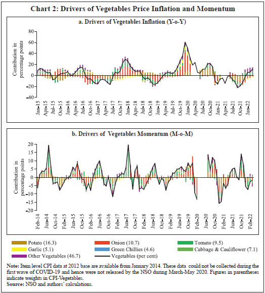 With such high contribution to variance of headline inflation, these three items warrant a closer scrutiny to assess likely build-up of price pressures in the near-term, as a sharp spike in their prices can derail the headline inflation from a stable trajectory. As already stated, India is the second largest producer of these vegetables in the world. However, while consumption of these items is ubiquitous, their production is concentrated in specific parts of the country under different agro-climatic conditions. 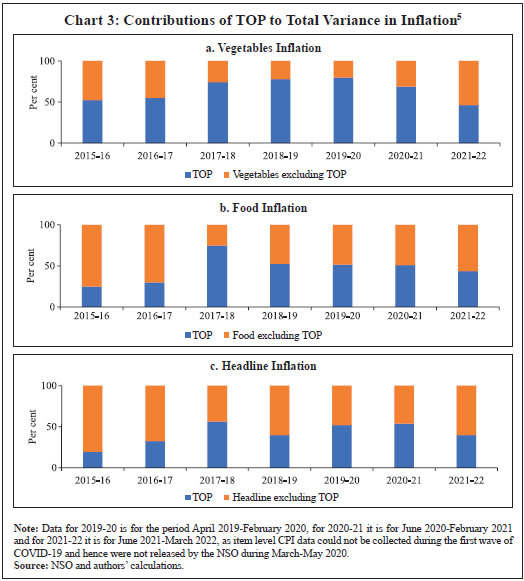 For instance, Maharashtra has the highest share in production of onions, while Madhya Pradesh and Uttar Pradesh are the leading producers of tomatoes and potatoes, respectively (Table 1). The top 5 states had a share of around 76 per cent, 50 per cent and 84 per cent in total production of onions, tomatoes and potatoes, respectively, during the period of 2017-18 to 2021-22. Such a skewed distribution of production indicates probable concentration of risk, emanating from adverse weather events or other supply shocks in these states, which could transmit to all over the country. Table 1: Top Five States by Production and Average Share in Production
(2017-18 to 2021-22) | | S. No. | Onion | Tomato | Potato | | State | % Share | State | % Share | State | % Share | | 1 | Maharashtra | 39.3 | Madhya Pradesh | 13.4 | Uttar Pradesh | 29.1 | | 2 | Madhya Pradesh | 16.1 | Andhra Pradesh | 12.6 | West Bengal | 24.6 | | 3 | Karnataka | 10.3 | Karnataka | 10.8 | Bihar | 16.1 | | 4 | Gujarat | 5.4 | Gujarat | 7.0 | Gujarat | 7.2 | | 5 | Bihar | 5.1 | Odisha | 6.6 | Madhya Pradesh | 6.6 | | Source: Department of Agriculture and Farmers Welfare, Ministry of Agriculture and Farmers Welfare. | Market arrivals of the TOP crops in the regional wholesale markets or “mandis” are therefore tracked to form a view about expected price movements in the near-term, such that lower/higher arrivals indicate higher/ lower prices (Chart 4 and Annex Table A8). Such information is available through various government sources like the Agmarknet portal, National Horticulture Board (NHB), National Horticultural Research and Development Foundation (NHRDF) and a few private agencies which track these items. Yet, with fruits and vegetables being delisted from the Agriculture Produce Market Committee (APMC) Act in many states, arrivals data from APMC mandis,may not indicate the true picture with respect to prices6. At the same time, another important source of price information for these items is the Department of Consumer Affairs (DCA) under the Ministry of Consumer Affairs, which collects daily data on prices of essential fooditems from 167 centres across the country7. In case of tomato, onion and potato, these prices have a high correlation of around 99 per cent with corresponding CPI indices (Annex Table A7). Thus, DCA data provide a good indication of price movement of these items for the current month as the data is released on a daily basis and can be used for nowcasting food inflation. But this data cannot be used for understanding the nature of price pressures, for which researchers often rely on news articles, announcements by ministry officials, information from traders and retailers and private agencies that track ground-level information for these commodities. This additional information on factors behind sudden price changes can be utilised to estimate the possible direction and duration of price shock and the magnitude of expected price changes.  Since TOP items have a high contribution to food inflation volatility and their prices are subject to supply shocks often induced by localised extreme weather events, farmers’ protests, transporters’ strikes, storage losses and sometimes speculative stocking by traders – all of which are covered by local newspapers – news articles related to TOP can provide additional information at an early stage of accumulating price pressures. Such information, which is usually in the form of unstructured data, can be used to create sentiment scores. If these commodity sentiments have lead information about future prices, they can be helpful in nowcasting and forecasting food inflation. Section III
Data and Methodology For the construction of a news-based sentiment indicator, we develop a novel dataset of daily news items related to TOP commodities from nine leading English news dailies published during January 2011 - August 2021. The newspapers are selected based on their national coverage and reporting on events and issues related to agri-commodities. In the first step, we use generic search terms, such as the name of a given commodity, to extract newsarticles related to a given commodity at scale8. Such text-mining applications are prone to ‘noise’ wherein articles unrelated to the topic of interest might also creep in, thereby lowering the signal-to-noise ratio of the data. Therefore, to avoid noise in the data, we create a set of keywords – ‘supply’, ‘demand’ and ‘prices’ – that capture the market dynamics of TOP commodities. We then filter and retain only those news items which contain at least one keyword each from the set of commodity, supply-demand and price-related keywords.9 This filtering step ensures that the dataset contains only the most contextual and meaningful information for our analysis, to the best extent possible (Chart 5). Finally, the text data are subjected to routine data cleaning procedure, such as removal of stopwords, numbers, white spaces and word stemming, etc., to organise the final dataset containing day-wise news items. 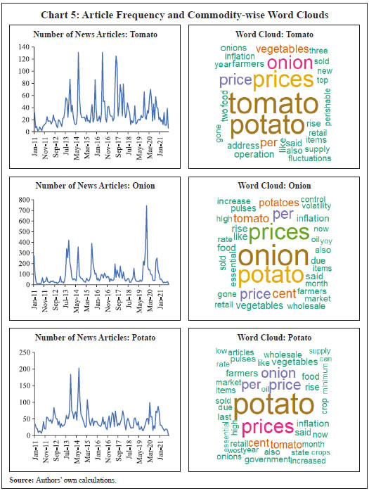 Next, we use the framework laid down by Ardia et al., (2021) for thecomputation of sentiment indices using newspaper text data10. While there are several approaches for sentiment computation, we adopt a lexicon-based approach, in particular a valence-shifting bigrams approach for the computation of commodity-wise sentiment indices. The lexicon-based approach is generally considered flexible, transparent, and computationally convenient as compared to other alternatives (Algaba et al., 2020). Briefly put, this approach matches words (or group of words) occurring in a document with a pre-defined wordlist of polarized (positive and negative) words and assigns quantitative scores to each matching word depending on whether its tonality is ‘positive’ or ‘negative’. For our purpose, the Loughran-McDonald lexicon – designed specifically for analysing economic and financial texts –was used (Loughran and McDonald, 2011)11. More specifically: 1. For each commodity-specific news item, the Loughran-McDonaldlexicon was used to assign a sentiment score {viSi,n,t} to each polarizedword occurring in a news article dn published at time t. The term vi captures the impact of valence shifters or keywords that may negate, amplify or de-amplify polarized words in the given document. 2. Thus, ‘positive’ and ‘negative’ words were assigned a sentiment score of (+1) and (-1), respectively. The scores were then adjusted for valence shifting words depending on whether such words appear before polarized words in the document. It may be noted that this computation occurs at the sentence-level to better account for such valence-shiftingkeywords12.
We assume that a positive (negative) sentiment score is indicative of an expected fall (increase) in the prices of the given commodity. This interpretation is corroborated by the analysis presented in the next section that sheds light on the historical relationship between our constructed sentiments and actual price movements of TOP commodities. Section IV
TOP Sentiment Indices - Preliminary Data Analysis TOP prices exhibit a seasonal pattern which is based on crop sowing and market arrivals across the country. However, they occasionally undergo major spikes due to localised factors, inducing high volatility to overall food inflation. The three vegetables were thus made part of essential commodities and were covered under the Essential Commodities Act, 1955 and hence their prices are monitored regularly by the government. Onion and potato, however, were removed from the list of essential commodities in September 2020 through an amendment to the Act with a rider that these items can be included in the list again only under extraordinary circumstances like wars, famines, or other natural calamities. As expected, the derived monthly net sentiment score of TOP and changes in their prices as reflected in CPI showcase an inverse relationshipbetween them13 (Chart 6). Large increases in TOP prices seen after major supply shocks coincide with large fall in sentiment related to each of the three commodities. Major price spikes observed in TOP in the recent past were often associated with supply shocks. During the period of our study i.e., from January 2011 to August 2021 (more than 10 years), tomato prices have undergone four major price spikes while both onion and potato have undergone five major price spikes.  The major causes of these sharp spikes include farmers’ protests, blight disease in potato, speculative stock holding by traders, heatwave, excess rains, etc., but the major and recurring source is related to weather related shocks. Unseasonal, excess or deficit rains affect the production of these perishable vegetables. The extent of price spikes, as measured by the month-on-month (m-o-m) change in CPI indices of these vegetables, i.e., momentum, indicate that the maximum spike was observed in tomato prices in July 2017 (138 per cent), which was the result of farmers’ protests in response to low prices of tomatoes being received by them. The extent of spikes in potato prices, however, is much lower compared to tomatoes and onions (maximum momentum of 31.4 per cent in November 2013). It can also be observed that the sharp spikes in prices usually last for one to two months in case of tomatoes and around three months in case of onions and potatoes. Given the importance of TOP, the government often resorts to supply management measures – like restricting exports, imposing condition of minimum export price (MEP), increasing imports, placing stockholding limits on traders, wholesalers and retailers – to ensure availability in the domestic market and stabilise prices. The inverse relationship between TOP prices as well as their sentiments is also corroborated by the pair-wise statistical correlations for the most recent five-year daily data sample from 2016-2021 (Table 2). For instance, while onion and potato prices have a correlation of 0.45, the correlation between their sentiments is 0.67. Similarly, correlation between prices of tomato with prices of potato and onion is 0.40 and 0.28, respectively, whereas related sentiments exhibit a much stronger correlation of 0.56 and 0.39, respectively. Correlation between the price-sentiment pair of tomato, onion and potato is (-)0.20, (-)0.42 and (-)0.33, respectively. Overall, the correlation between TOP sentiments and prices is negative signifying that a decrease in TOP sentiments is associated with an increase in related prices. | Table 2: Price-Sentiment Correlation Matrix | | Correlation | Tomato Price | Onion Price | Potato Price | Tomato Sentiment | Onion Sentiment | Potato Sentiment | | Tomato Price | 1.00 | | | | | | | Onion Price | 0.28*** | 1.00 | | | | | | Potato Price | 0.40*** | 0.45*** | 1.00 | | | | | Tomato Sentiment | -0.20*** | 0.02 | -0.11 | 1.00 | | | | Onion Sentiment | -0.09 | -0.42*** | -0.36*** | 0.39*** | 1.00 | | | Potato Sentiment | -0.06 | -0.21*** | -0.33*** | 0.56*** | 0.67*** | 1.00 | Note: 1. * p < 0.1, ** p < 0.05, *** p < 0.01 denotes the level of significance.
2. The above analysis uses 30-day daily moving average of prices/sentiments.
Source: Authors’ own calculations. | As a next step, we subject the daily TOP prices and sentiment indices to a Granger Causality test to ascertain whether news-based sentiments are helpful in capturing the change in prices. Our results show that sentiment Granger causes prices for all the three commodities supporting the argument that the constructed sentiment indices are indeed helpful in capturing the future change in prices (Table 3). | Table 3: Price-Sentiment Granger Causality Test | | Variable | H01: Price does not Granger cause sentiment | H02: Sentiment does not Granger cause price | | Potato | 0.108 | 0.003*** | | Onion | 0.401 | 0.000*** | | Tomato | 0.678 | 0.000*** | Note: * p < 0.10, ** p < 0.05, *** p < 0.01 denotes the level of significance.
Source: Author’s own calculations. | Section V
Empirical Analysis The preliminary statistical analysis in the previous sections is indicative of useful forward-looking information contained in the commodity sentiment indices. To formally analyse this, we undertake a time-series forecasting analysis. This section lays down the details of our forecasting analysis conducted using monthly and daily high-frequency data. In the first part of our forecasting analysis, we augment various univariate and multivariate time-series models with our sentiment indices and test their forecasting performance against a benchmark model. Like the news-based sentiment data, DCA provides an alternative set of high-frequency information on prices of food commodities across different centres in India. This data can be regarded as ‘hard’ information which can also be used in inflation projections. Therefore, the second part of our analysis focuses on comparing the forecasting performance of models augmented with sentiment data vis-à-vis DCA price data for TOP commodities. In the final part of our analysis, we showcase how daily high-frequency sentiment indices can be used to forecast CPI-Food inflation in a mixed-frequency sample framework. V.1. Forecasting using Monthly Data For the formal forecasting analysis, we consider monthly changes in CPI-Vegetables and CPI-Food & beverages, both in month-on-month (m-o-m) and year-on-year (y-o-y) per cent change terms, as our target variables. Thus, we have four different target variables. In line with standard practice, we divide the full sample of data into a training and a testing sample. The train sample, from January 2011 to August 2019, was used for estimation of the models. The test sample, from September 2019 to August 2021, was used for comparing model forecast performance in terms of the root mean-squared error (RMSE) of forecasts generated by different models. We consider different specifications of autoregressive integrated movingaverage (ARIMA) models14. Taking the approach of parsimony, we combine all TOP-related news articles and use the sentiment scoring method described in section III to construct a composite TOP sentiment index. We introduce this index into our suite of ARIMA models to assess whether inclusion of such news-based information leads to gains in forecasting accuracy. Following Jose et al., (2021), other drivers of domestic food prices, such as global food prices, rainfall and minimum support prices (MSP), were also included as control variables in the forecasting model for robustness (additional results provided in the Appendix). The out-of-sample forecast performance of various models is provided in Tables 4-7. To capture the performance of models augmented with sentiment data over time, we combine the standard out-of-sample forecasting approach with a rolling window to ensure a dynamic and robust evaluation of model forecast performance across horizons. For ease of comparison, we present the results in terms of relative performance vis-à-vis a benchmark AR(1) model, where relative performance is defined as RMSE of model m at horizon h scaled by the RMSE of the benchmark model for the same horizon. Any value less than one suggests gains in forecasting accuracy as it indicates that the actual RMSE value for a given model is lower than that of the benchmark model. Beginning with Table 4, which presents results for the m-o-m changes in CPI-Vegetables series, almost all models from M2-M6, are able to outperform the benchmark AR model (M1) across different horizons, particularly less than 6-months. However, addition of sentiment data is seen to improve forecasting performance across all horizons. For instance, augmenting a simple AR(1) model with NSS (M2) results in forecasting gains of about 2-6 per cent across horizons. Similarly, adding NSS to seasonal ARIMA model (M6 vs. M5) leads to better forecast performance, such that M6 is able to generate accuracy gains to the tune of 7-10 per cent over the benchmark across horizons. | Table 4: Rolling-window Out-of-Sample Forecasting Performance CPI-Vegetables (m-o-m, per cent) | | Model/Description | Forecast Horizon (in months) | | 1 | 2 | 3 | 4 | 5 | 6 | 7 | 8 | 9 | 10 | 11 | 12 | | M1 AR(1) | 1.00 | 1.00 | 1.00 | 1.00 | 1.00 | 1.00 | 1.00 | 1.00 | 1.00 | 1.00 | 1.00 | 1.00 | | M2 AR(1) + NSS | 0.95 | 0.94 | 0.95 | 0.96 | 0.96 | 0.97 | 0.98 | 0.98 | 0.98 | 0.98 | 0.98 | 0.97 | | M3 ARIMA | 0.99 | 0.96 | 0.99 | 1.00 | 0.99 | 1.00 | 1.00 | 1.00 | 1.00 | 1.00 | 1.00 | 1.00 | | M4 ARIMA + NSS | 0.96 | 0.93 | 0.97 | 0.98 | 0.97 | 0.98 | 0.99 | 0.99 | 0.99 | 0.98 | 0.98 | 0.98 | | M5 SARIMA | 0.95 | 0.92 | 0.95 | 0.96 | 0.95 | 0.96 | 0.95 | 0.96 | 0.96 | 0.96 | 0.95 | 0.95 | | M6 SARIMA + NSS | 0.93 | 0.90 | 0.93 | 0.94 | 0.94 | 0.95 | 0.95 | 0.95 | 0.95 | 0.94 | 0.93 | 0.94 | Note: The table shows the relative RMSE of each model m for horizon h measured over the test sample. The AR(1) model is taken as the benchmark model. NSS refers to the TOP Net Sentiment Score Index.
Source: Authors’ own calculations. |
| Table 5: Rolling-window Out-of-Sample Forecasting Performance CPI-Vegetables (y-o-y, per cent) | | Model/Description | Forecast Horizon (in months) | | 1 | 2 | 3 | 4 | 5 | 6 | 7 | 8 | 9 | 10 | 11 | 12 | | M1 AR(1) | 1.00 | 1.00 | 1.00 | 1.00 | 1.00 | 1.00 | 1.00 | 1.00 | 1.00 | 1.00 | 1.00 | 1.00 | | M2 AR(1) + NSS | 0.99 | 0.99 | 0.99 | 0.99 | 0.99 | 0.99 | 0.98 | 0.98 | 0.98 | 0.99 | 0.99 | 0.99 | | M3 ARIMA | 0.99 | 1.04 | 0.99 | 0.96 | 0.97 | 0.93 | 0.95 | 0.96 | 1.04 | 1.05 | 0.89 | 0.73 | | M4 ARIMA + NSS | 0.99 | 1.04 | 0.99 | 0.96 | 0.97 | 0.93 | 0.94 | 0.95 | 1.03 | 1.03 | 0.88 | 0.72 | | M5 SARIMA | 0.77 | 0.92 | 0.95 | 0.93 | 0.95 | 0.98 | 1.09 | 1.07 | 0.89 | 0.74 | 0.56 | 0.53 | | M6 SARIMA + NSS | 0.79 | 0.91 | 0.97 | 0.97 | 0.98 | 1.03 | 1.08 | 1.01 | 0.90 | 0.72 | 0.58 | 0.55 | Note: The table shows the relative RMSE of each model m for horizon h measured over the test sample, where an AR(1) model is taken as the benchmark model. A relative RMSE value of less than 1 indicates improvement in forecasting accuracy. NSS refers to the composite TOP Sentiment Index.
Source: Authors’ own calculations. | Forecasting performance in case of y-o-y measure of CPI-Vegetables showcases the benefits of incorporating news-based information even further, especially at the near-term horizon (Table 5). While not much improvement is seen in case of ARIMA models (M2-M4), SARIMA models deliver better forecast performance. The forecasting performance of models for the m-o-m changes in CPI-Food and beverages, however, are mixed (Table 6). The AR(1) model augmented with NSS delivers better forecast performance compared to the benchmark model, although these gains are comparatively modest (2-5 per cent) relative to CPI-Vegetables. Rest of the models fails to outperform the benchmark. | Table 6: Rolling-window Out-of-Sample Forecasting Performance CPI-Food & beverages (m-o-m, per cent) | | Model/Description | Forecast Horizon (in months) | | 1 | 2 | 3 | 4 | 5 | 6 | 7 | 8 | 9 | 10 | 11 | 12 | | M1 AR(1) | 1.00 | 1.00 | 1.00 | 1.00 | 1.00 | 1.00 | 1.00 | 1.00 | 1.00 | 1.00 | 1.00 | 1.00 | | M2 AR(1) + NSS | 0.96 | 0.95 | 0.96 | 0.97 | 0.97 | 0.97 | 0.98 | 0.98 | 0.98 | 0.98 | 0.97 | 0.96 | | M3 ARIMA | 1.08 | 1.12 | 1.17 | 1.09 | 1.11 | 1.08 | 1.13 | 1.05 | 1.07 | 1.05 | 1.08 | 1.10 | | M4 ARIMA + NSS | 1.06 | 0.98 | 1.02 | 0.99 | 1.01 | 1.02 | 1.04 | 1.05 | 1.01 | 1.01 | 1.00 | 1.02 | | M5 SARIMA | 1.05 | 1.00 | 1.08 | 1.00 | 1.05 | 1.03 | 1.01 | 1.04 | 0.99 | 1.01 | 1.07 | 1.16 | | M6 SARIMA + NSS | 1.06 | 0.98 | 1.02 | 0.99 | 1.01 | 1.02 | 1.04 | 1.05 | 1.01 | 1.01 | 1.00 | 1.02 | Note: The table shows the relative RMSE of each model m for horizon h measured over the test sample, where an AR(1) model is taken as the benchmark model. A relative RMSE value of less than 1 indicates improvement in forecasting accuracy. NSS refers to the composite TOP Sentiment Index.
Source: Authors’ own calculations. | Lastly, in case of CPI-Food and beverages y-o-y series, SARIMA model (M5) and SARIMA model with sentiment information (M6) provides the best forecasts (Table 7). As seen in the earlier cases, adding sentiment information to forecasting models leads to a general improvement in forecasting accuracy. V.2. Forecast Comparison between Sentiment data and DCA Data To compare the extent of forward-looking information embedded in news-based ‘soft’ data and ‘hard’ DCA data, we estimate separate bivariate vector autoregression (VAR) models containing each set of indicators and compare their out-of-sample forecasting performance. A bivariate VAR model can be generally expressed as follows: where yi,t represents a set of endogenous variables whereas Ɛ1,t and Ɛ2,t are white noise processes that may be contemporaneously correlated. Our basic framework, including the target indicators, forecast horizon and train-test sample, remains the same as in the last subsection15. We estimate the VAR model using ordinary least squares (OLS) method while choosing optimal lag structure via the AIC criterion. The forecasting performance based on rolling out-of-sample forecasts, in the form of relative RMSE with respect to a benchmark AR(1) model, is provided in Table 8. Table 7: Rolling-window Out-of-Sample Forecasting Performance CPI-Food & beverages (y-o-y, per cent) | | Model/Description | Forecast Horizon (in months) | | 1 | 2 | 3 | 4 | 5 | 6 | 7 | 8 | 9 | 10 | 11 | 12 | | M1 AR(1) | 1.00 | 1.00 | 1.00 | 1.00 | 1.00 | 1.00 | 1.00 | 1.00 | 1.00 | 1.00 | 1.00 | 1.00 | | M2 AR(1) + NSS | 0.98 | 0.99 | 0.99 | 0.98 | 0.98 | 0.99 | 0.99 | 0.99 | 0.99 | 0.99 | 0.99 | 0.98 | | M3 ARIMA | 1.02 | 1.01 | 1.00 | 0.95 | 0.96 | 0.95 | 0.93 | 0.93 | 0.92 | 0.89 | 0.84 | 0.88 | | M4 ARIMA + NSS | 0.99 | 1.00 | 1.00 | 0.96 | 0.95 | 0.96 | 0.94 | 0.93 | 0.92 | 0.90 | 0.84 | 0.86 | | M5 SARIMA | 0.76 | 0.74 | 0.74 | 0.72 | 0.72 | 0.70 | 0.73 | 0.74 | 0.66 | 0.57 | 0.55 | 0.58 | | M6 SARIMA + NSS | 0.76 | 0.74 | 0.74 | 0.72 | 0.72 | 0.71 | 0.73 | 0.74 | 0.66 | 0.57 | 0.55 | 0.58 | Note: The table shows the relative RMSE of each model m for horizon h measured over the test sample, where an AR(1) model is taken as the benchmark model. A relative RMSE value of less than 1 indicates improvement in forecasting accuracy. NSS refers to the composite TOP Sentiment Index.
Source: Authors’ own calculations. | In case of CPI-Vegetables inflation, both set of indicators showcase a similar forecasting ability across time horizons. In some cases, such as m-o-m CPI-Vegetables model augmented with sentiment or DCA data fail to outperform the benchmark. However, in case of CPI-Food & beverages inflation, bivariate VAR model with sentiment data outperforms both the benchmark and DCA data-based model across horizons. In case of m-o-m measure, the gains in forecasting accuracy range from 13 to 32 per cent, whereas even higher gains ranging from 56 to 75 per cent accrue when sentiment data is used to forecast the CPI-Food & beverages y-o-y measure of inflation. This highlights the efficacy of sentiment data for forecasting inflation over and above the only other existing high-frequency prices data provided by DCA. | Table 8: Forecasting Performance – Sentiment vs. DCA data | | Model/Description | Forecast Horizon (in months) | | 1 | 2 | 3 | 4 | 5 | 6 | 7 | 8 | 9 | 10 | 11 | 12 | | CPI-Vegetables (m-o-m, per cent) | | M1 AR(1) | 1.00 | 1.00 | 1.00 | 1.00 | 1.00 | 1.00 | 1.00 | 1.00 | 1.00 | 1.00 | 1.00 | 1.00 | | M2 VAR with DCA | 1.02 | 0.98 | 0.99 | 0.99 | 1.01 | 1.00 | 1.02 | 1.02 | 1.01 | 1.01 | 1.02 | 1.01 | | M3 VAR with NSS | 0.99 | 0.97 | 0.99 | 1.00 | 1.00 | 1.00 | 1.02 | 1.02 | 1.01 | 1.01 | 1.02 | 1.01 | | CPI-Vegetables (y-o-y, per cent) | | M1 AR(1) | 1.00 | 1.00 | 1.00 | 1.00 | 1.00 | 1.00 | 1.00 | 1.00 | 1.00 | 1.00 | 1.00 | 1.00 | | M2 VAR with DCA | 0.98 | 1.00 | 0.92 | 0.88 | 0.86 | 0.87 | 0.89 | 0.93 | 0.98 | 0.97 | 0.85 | 0.77 | | M3 VAR with NSS | 0.97 | 0.99 | 0.92 | 0.89 | 0.89 | 0.88 | 0.93 | 0.96 | 1.01 | 0.99 | 0.87 | 0.77 | | CPI-Food & beverages (m-o-m, per cent) | | M1 AR(1) | 1.00 | 1.00 | 1.00 | 1.00 | 1.00 | 1.00 | 1.00 | 1.00 | 1.00 | 1.00 | 1.00 | 1.00 | | M2 VAR with DCA | 1.04 | 0.98 | 0.99 | 0.99 | 1.00 | 1.00 | 1.01 | 1.01 | 1.00 | 1.00 | 1.02 | 1.01 | | M3 VAR with NSS | 0.68 | 0.66 | 0.69 | 0.70 | 0.70 | 0.70 | 0.80 | 0.80 | 0.84 | 0.87 | 1.07 | 1.14 | | CPI-Food & beverages (y-o-y, per cent) | | M1 AR(1) | 1.00 | 1.00 | 1.00 | 1.00 | 1.00 | 1.00 | 1.00 | 1.00 | 1.00 | 1.00 | 1.00 | 1.00 | | M2 VAR with DCA | 1.00 | 1.01 | 0.97 | 0.92 | 0.94 | 0.96 | 0.95 | 0.97 | 0.99 | 0.97 | 0.89 | 0.91 | | M3 VAR with NSS | 0.44 | 0.29 | 0.27 | 0.25 | 0.26 | 0.28 | 0.29 | 0.28 | 0.31 | 0.30 | 0.28 | 0.26 | Note: The table shows the relative RMSE of each model m for horizon h measured over the test sample, where an AR(1) model is taken as the benchmark model. A relative RMSE value of less than 1 indicates improvement in forecasting accuracy. NSS refers to the composite TOP Sentiment Index.
Source: Authors’ calculations. | V.3. Forecasting using Mixed-frequency Data: A MIDAS Approach Having access to high-frequency news data, we exploit the information embedded in daily news sentiments to forecast monthly inflation series. A mixed data sampling (MIDAS) regression approach comes in handy by allowing the use of data sampled at different frequencies in the same regression. In particular, the MIDAS methodology proposed by Ghysels et al. (2002; 2006; 2007) and Andreou et al. (2010) allows the estimation of regression models where the dependent variable is sampled at a lower frequency compared to one or more of the independent variables. Thus, MIDAS helps in incorporating the information in higher-frequency data into the lower frequency regression model in a flexible and parsimonious way. A MIDAS regression model can be generally specified as follows: 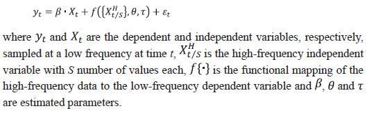 Traditional approaches to mixed-frequency regression either introduce a sum/average of the high-frequency data with a single coefficient (implicitly equal weights) or include individual components of the high-frequency variable in the model allowing for separate coefficients. On the other hand, by allowing for several different weighting functions to decide optimal weights and reducing the number of estimated parameters by placing adequate constraints, the MIDAS approach offers a flexible framework to incorporate high-frequency information into a regression model. Various weighting schemes available under this approach are (a) step-weighting; (b) polynomial distributed lag (PDL) weighting; (c) exponential PDL weighting; (d) normalised beta function weighting; and (e) individual coefficients weighting technique (U-MIDAS). Adopting a similar train-test approach as in the previous sub-section, we use a simple AR(1) model estimated using the MIDAS framework with PDL and U-MIDAS weighting techniques for predicting our target variable. We incorporate the high-frequency information by introducing up to 30 lags of combined TOP net sentiment score computed at a daily frequency. The out-of-sample forecasts on test data are generated using the dynamic rolling window approach from one-to 12-months ahead horizon. The forecast performance, in the form of relative RMSE of forecasts generated by best-performing MIDAS model compared to the AR(1) benchmark, is presented in Table 9. | Table 9: Mixed-frequency Forecasting Target: CPI-Vegetables/CPI-Food & Beverages | | Model | Forecast Horizon (in months) | | 1 | 2 | 3 | 4 | 5 | 6 | 7 | 8 | 9 | 10 | 11 | 12 | | CPI-Vegetables (m-o-m, per cent) | | M1 AR(1) | 1.00 | 1.00 | 1.00 | 1.00 | 1.00 | 1.00 | 1.00 | 1.00 | 1.00 | 1.00 | 1.00 | 1.00 | | M2 MIDAS: AR(1) + Daily NSS | 0.95 | 0.96 | 0.98 | 0.97 | 0.98 | 0.98 | 1.00 | 1.00 | 1.00 | 0.99 | 1.02 | 1.05 | | CPI-Vegetables (y-o-y, per cent) | | M1 AR(1) | 1.00 | 1.00 | 1.00 | 1.00 | 1.00 | 1.00 | 1.00 | 1.00 | 1.00 | 1.00 | 1.00 | 1.00 | | M2 MIDAS: AR(1) + Daily NSS | 1.00 | 0.99 | 1.00 | 1.00 | 1.00 | 1.04 | 1.11 | 1.14 | 1.20 | 1.21 | 1.15 | 1.09 | | CPI-Food & beverages (m-o-m, per cent) | | M1 AR(1) | 1.00 | 1.00 | 1.00 | 1.00 | 1.00 | 1.00 | 1.00 | 1.00 | 1.00 | 1.00 | 1.00 | 1.00 | | M2 MIDAS: AR(1) + Daily NSS | 0.96 | 0.96 | 0.97 | 0.97 | 0.98 | 0.98 | 0.99 | 0.98 | 0.99 | 0.98 | 1.02 | 1.05 | | CPI-Food & beverages (y-o-y, per cent) | | M1 AR(1) | 1.00 | 1.00 | 1.00 | 1.00 | 1.00 | 1.00 | 1.00 | 1.00 | 1.00 | 1.00 | 1.00 | 1.00 | | M2 MIDAS: AR(1) + Daily NSS | 1.01 | 1.08 | 1.19 | 1.26 | 1.28 | 1.31 | 1.28 | 1.19 | 1.20 | 1.22 | 1.18 | 1.18 | Note: The table shows the relative RMSE of each model m for horizon h measured over the test sample, where an AR(1) model is taken as the benchmark model. A relative RMSE value of less than 1 indicates improvement in forecasting accuracy. NSS refers to the composite TOP Sentiment Index.
Source: Authors’ own calculations. | As is evident from Table 9, leveraging daily news-based sentiment data has clear benefits in terms of gains in forecasting accuracy in m-o-m space. In case of m-o-m changes in CPI-Vegetables and CPI-Food and beverages, the MIDAS model with daily data outperforms the benchmark model at the one-month ahead horizon. In addition to these one-month ahead predictions or nowcasts, the MIDAS model outperforms the benchmark for two- to six-months ahead horizon, where the gains range from 2-5 per cent for m-o-m changes in CPI-Vegetables and CPI-Food and beverages series. On the other hand, sentiment augmented model fails to outperform the benchmark model in case of inflation measures taken in y-o-y terms across different horizons. Thus, overall, it can be said that daily news-based sentiment indicators for TOP commodities can help near-term month-on-month projections of price index for CPI Vegetables and CPI Food and beverages over different forecast horizons. Section VI
Conclusion and the Way Forward Recurrent supply disruptions driven by unseasonal rainfall, floods, droughts, pest attacks, protests by farmers/transport operators, etc., makes the task of inflation forecasting an arduous challenge in India. In this study, therefore, we develop a novel dataset consisting of news articles related to three main agricultural commodities viz., tomato, onion and potato or TOP to forecast CPI-based inflation in vegetables and food & beverages. We quantify the information content of news articles using natural language processing (NLP) techniques to assess whether news-based alternate data can help in achieving better forecasts. Through various forecasting methods premised on monthly and daily data, we provide empirical evidence to conclude that news-based data in the form of sentiment indices provides gains in forecasting accuracy. The forward-looking information content embedded in news data, therefore, suggests the use of news-based sentiment indicators as an additional source of information for inflation forecasting. This is crucial from a policy perspective in an environment of highly uncertain food price dynamics that are increasingly becoming climate dependent. While this study is a first step in the direction of using news-based big data for food inflation forecasting, the analysis can be extended in several ways. From the perspective of forecasting headline inflation and its components, a larger number of commodities and other items corresponding with the official CPI basket can be included in the forecasting framework. More nuanced NLP techniques, such as those based on supervised machine-learning methods for sentiment quantification, or unsupervised topic modelling approach can be used to derive more granular information on topics such as supply and demand for various items. The suite of time-series methods can also be expanded to experiment with other advanced techniques, such as dynamic factor models, penalized regressions and deep learning models which might help achieve better forecasting accuracy. Moreover, given the forward-looking content of news-based data, it can also be used for turning point analysis of inflationary shocks to the economy. Finally, while we have focused on point forecasts in this paper, it remains to be seen whether news-based information can also help in reducing the uncertainty around forecasts. We leave these issues for future research.
References Aprigliano, V., Emiliozzi, S., Guaitoli, G., Luciani, A., Marcucci, J., & Monteforte, L. (2022). The power of text-based indicators in forecasting Italian economic activity. International Journal of Forecasting. Algaba, A., Ardia, D., Bluteau, K., Borms, S., & Boudt, K. (2020). Econometrics meets sentiment: An overview of methodology and applications. Journal of Economic Surveys, 34(3), 512-547. Andreou, E., Ghysels, E., & Kourtellos, A. (2013). Should macroeconomic forecasters use daily financial data and how? Journal of Business & Economic Statistics, 31(2), 240-251. Ardia, D., Bluteau, K., Borms, S., & Boudt, K. (2021). The R package sentometrics to compute, aggregate and predict with textual sentiment. Journal of Statistical Software, 99(2), 1-40. Banerjee, A., Kanodia, A., & Ray, P. (2021). Deciphering Indian inflationary expectations through text mining: an exploratory approach. Indian Economic Review, 1-18. Barbaglia, L., Consoli, S., & Manzan, S. (2022). Forecasting with economic news. Journal of Business & Economic Statistics, 1-12. Bholat, D., Hansen, S., Santos, P., & Schonhardt-Bailey, C. (2015). Text mining for central banks. Available at SSRN 2624811. Ellingsen, J., Larsen, V. H., & Thorsrud, L. A. (2022). News media versus FRED-MD for macroeconomic forecasting. Journal of Applied Econometrics, 37(1), 63-81. Gandomi, A., & Haider, M. (2015). Beyond the hype: Big data concepts, methods, and analytics. International Journal of Information Management, 35(2), 137-144. Gentzkow, M., Kelly, B., & Taddy, M. (2019). Text as data. Journal of Economic Literature, 57(3), 535-74. Ghosh, S. , Kundu, S., & Dilip, A. (2021). Green Swans and their Economic Impact on Indian Coastal States. Reserve Bank of India Occasional Papers, 42(1). Ghysels, E., Santa-Clara, P., & Valkanov, R. (2002). The MIDAS touch: Mixed data sampling regression models. Working Paper, UNC and UCLA. Ghysels, E., Santa-Clara, P., & Valkanov, R. (2006). Predicting volatility: getting the most out of return data sampled at different frequencies. Journal of Econometrics, 131(1-2), 59-95. Ghysels, E., Sinko, A., & Valkanov, R. (2007). MIDAS regressions: Further results and new directions. Econometric Reviews, 26(1), 53-90. Goshima, K., Ishijima, H., Shintani, M., & Yamamoto, H. (2021). Forecasting Japanese inflation with a news-based leading indicator of economic activities. Studies in Nonlinear Dynamics & Econometrics, 25(4), 111-133. John, J., Singh, S., & Kapur, M. (2020). Inflation forecast combinations – The Indian experience. RBI Working Paper Series, No. 11/2020, Reserve Bank of India, Mumbai, India. Jose, J., Shekhar, H., Kundu, S., Kishore, V., & Bhoi, B. B. (2021). Alternative Inflation Forecasting Models for India–What Performs Better in Practice?. Reserve Bank of India Occasional Papers, 42(1). Kalamara, E., Turrell, A., Redl, C., Kapetanios, G., & Kapadia, S. (2020). Making Text Count: Economic Forecasting Using Newspaper Text. Bank of England Working Paper No. 865, Available at SSRN: https://ssrn.com/abstract=3610770 or http://dx.doi.org/10.2139/ssrn.3610770 Kapur, M. (2013). Revisiting the Phillips curve for India and inflation forecasting. Journal of Asian Economics. 25(1), 17-27 Kishore, V. and Shekhar, H. (2022), Extreme weather events and vegetables inflation in India. Economic and Political Weekly. Forthcoming. Kumari, S., & Giddi, G. (2020). Inflation decoded through the power of words. RBI Monthly Bulletin, May, Reserve Bank of India, Mumbai, India. Larsen, V. H., & Thorsrud, L. A. (2019). The value of news for economic developments. Journal of Econometrics, 210(1), 203-218. Lei, C., Lu, Z., & Zhang, C. (2015). News on inflation and the epidemiology of inflation expectations in China. Economic Systems, 39(4), 644-653. Liu, B. (2020). Sentiment analysis: Mining opinions, sentiments, and emotions. Cambridge University Press. Loughran, T., & McDonald, B. (2011). When is a liability not a liability? Textual analysis, dictionaries, and 10-Ks. The Journal of Finance, 66(1), 35-65. Maji, B., & Das, A. (2016). Forecasting inflation with mixed frequency data in India. Calcutta Statistical Association Bulletin, 68(1-2), 92-110. Munezero, M., Montero, C. S., Sutinen, E., & Pajunen, J. (2014). Are they different? Affect, feeling, emotion, sentiment, and opinion detection in text. IEEE Transactions on Affective Computing, 5(2), 101-111. Priyaranjan, N., & Pratap, B. (2020). Macroeconomic Effects of Uncertainty: A Big Data Analysis for India. RBI Working Paper Series (No. 04/2020), Reserve Bank of India, Mumbai, India. Pratap, B., & Sengupta, S. (2019). Macroeconomic forecasting in India: Does machine learning hold the key to better forecasts?. RBI Working Paper Series, No. 04/2019, Reserve Bank of India, Mumbai, India. Rambaccussing, D., & Kwiatkowski, A. (2020). Forecasting with news sentiment: Evidence with UK newspapers. International Journal of Forecasting, 36(4), 1501-1516. Ravi, K., & Ravi, V. (2015). A survey on opinion mining and sentiment analysis: tasks, approaches and applications. Knowledge-based Systems, 89, 14-46. Reserve Bank of India. (2021). Monetary Policy Report, October. Sahoo, S., Kumar S. and Gupta B. (2020). Pass-through of international food prices to emerging market economies: A revisit. Reserve Bank of India Occasional Papers, Vol. 41, No. 1: 2020 Sahu, S., & Chattopadhyay, S. (2020). Epidemiology of inflation expectations and internet search: an analysis for India. Journal of Economic Interaction and Coordination, 15(3), 649-671. Shapiro, A. H., Sudhof, M., & Wilson, D. J. (2020). Measuring news sentiment. Journal of Econometrics, 228 (2), 221-243. Taboada, M. (2016). Sentiment analysis: An overview from linguistics. Annual Review of Linguistics, 2, 325-347. Thakur, G. S. M., Bhattacharyya, R., & Mondal, S. S. (2016). Artificial neural network-based model for forecasting of inflation in India. Fuzzy Information and Engineering, 8(1), 87-100. Tilly, S., Ebner, M., & Livan, G. (2021). Macroeconomic forecasting through news, emotions and narrative. Expert Systems with Applications, 175, 114760.
Appendix | Table A1: Rolling-window Out-of-Sample Forecasting Performance - CPI-Vegetables (m-o-m, per cent) | | Model/Description | Forecast Horizon (in months) | | 1 | 2 | 3 | 4 | 5 | 6 | 7 | 8 | 9 | 10 | 11 | 12 | | M1 AR(1) | 6.49 | 6.77 | 6.65 | 6.72 | 6.84 | 6.85 | 5.79 | 5.91 | 5.64 | 5.70 | 5.62 | 5.02 | | M2 AR(1) + NSS | 6.15 | 6.34 | 6.34 | 6.46 | 6.55 | 6.64 | 5.69 | 5.79 | 5.54 | 5.56 | 5.49 | 4.87 | | M3 ARIMA | 6.44 | 6.47 | 6.59 | 6.72 | 6.78 | 6.84 | 5.80 | 5.92 | 5.65 | 5.72 | 5.63 | 5.02 | | M4 ARIMA + NSS | 6.25 | 6.33 | 6.44 | 6.57 | 6.65 | 6.74 | 5.75 | 5.85 | 5.58 | 5.61 | 5.53 | 4.94 | | M5 SARIMA | 6.16 | 6.20 | 6.32 | 6.44 | 6.53 | 6.58 | 5.51 | 5.67 | 5.40 | 5.47 | 5.32 | 4.79 | | M6 SARIMA + NSS | 6.01 | 6.08 | 6.20 | 6.31 | 6.42 | 6.50 | 5.48 | 5.62 | 5.34 | 5.38 | 5.23 | 4.73 | | M7 SARIMA + Exo | 6.19 | 6.38 | 6.45 | 6.55 | 6.69 | 6.70 | 5.81 | 5.93 | 5.47 | 5.52 | 5.63 | 5.28 | | M8 SARIMA +Exo + NSS | 6.14 | 6.30 | 6.38 | 6.46 | 6.58 | 6.59 | 5.68 | 5.78 | 5.35 | 5.41 | 5.49 | 5.20 | Note: The table shows the RMSE of each model m for horizon h measured over the test sample. The AR(1) model is taken as the benchmark model. Exo refers to exogenous variables such as global food prices, rainfall and minimum support prices (MSP) while NSS refers to the composite TOP Sentiment Index.
Source: Authors’ own calculations. |
| Table A2: Rolling-window Out-of-Sample Forecasting Performance - CPI-Vegetables (y-o-y, per cent) | | Model/Description | Forecast Horizon (in months) | | 1 | 2 | 3 | 4 | 5 | 6 | 7 | 8 | 9 | 10 | 11 | 12 | | M1 AR(1) | 11.14 | 16.80 | 19.47 | 21.06 | 19.81 | 17.09 | 15.29 | 15.17 | 14.03 | 14.67 | 17.36 | 20.41 | | M2 AR(1) + NSS | 11.08 | 16.69 | 19.26 | 20.81 | 19.60 | 16.88 | 14.98 | 14.93 | 13.80 | 14.47 | 17.25 | 20.28 | | M3 ARIMA | 11.06 | 17.40 | 19.29 | 20.28 | 19.13 | 15.95 | 14.49 | 14.59 | 14.64 | 15.34 | 15.45 | 14.84 | | M4 ARIMA + NSS | 11.05 | 17.44 | 19.37 | 20.31 | 19.13 | 15.89 | 14.37 | 14.46 | 14.49 | 15.17 | 15.30 | 14.68 | | M5 SARIMA | 8.63 | 15.40 | 18.55 | 19.64 | 18.88 | 16.67 | 16.69 | 16.18 | 12.55 | 10.79 | 9.77 | 10.74 | | M6 SARIMA + NSS | 8.76 | 15.23 | 18.79 | 20.34 | 19.49 | 17.59 | 16.56 | 15.31 | 12.61 | 10.56 | 10.11 | 11.19 | | M7 SARIMA + Exo. | 4.99 | 6.05 | 9.00 | 9.57 | 10.98 | 12.44 | 13.69 | 13.57 | 14.21 | 14.73 | 15.08 | 14.95 | | M8 SARIMA+ Exo+NSS | 2.94 | 5.33 | 8.80 | 9.71 | 11.20 | 12.90 | 14.60 | 15.11 | 15.07 | 15.51 | 16.18 | 16.46 | Note: The table shows the RMSE of each model m for horizon h measured over the test sample. The AR(1) model is taken as the benchmark model. Exo refers to exogenous variables such as global food prices, rainfall and minimum support prices (MSP) while NSS refers to the composite TOP Sentiment Index.
Source: Authors’ own calculations. |
| Table A3: Rolling-window Out-of-Sample Forecasting Performance - CPI-Food & Beverages (m-o-m, per cent) | | Model/Description | Forecast Horizon (in months) | | 1 | 2 | 3 | 4 | 5 | 6 | 7 | 8 | 9 | 10 | 11 | 12 | | M1 AR(1) | 1.27 | 1.27 | 1.26 | 1.26 | 1.29 | 1.29 | 1.14 | 1.18 | 1.14 | 1.14 | 0.95 | 0.87 | | M2 AR(1) + NSS | 1.21 | 1.21 | 1.21 | 1.22 | 1.24 | 1.26 | 1.12 | 1.15 | 1.12 | 1.12 | 0.92 | 0.84 | | M3 ARIMA | 1.37 | 1.42 | 1.48 | 1.37 | 1.43 | 1.39 | 1.29 | 1.24 | 1.22 | 1.20 | 1.02 | 0.96 | | M4 ARIMA + NSS | 1.34 | 1.25 | 1.29 | 1.24 | 1.29 | 1.32 | 1.18 | 1.23 | 1.15 | 1.14 | 0.95 | 0.89 | | M5 SARIMA | 1.33 | 1.28 | 1.36 | 1.27 | 1.35 | 1.33 | 1.15 | 1.22 | 1.13 | 1.14 | 1.01 | 1.01 | | M6 SARIMA + NSS | 1.34 | 1.25 | 1.29 | 1.24 | 1.29 | 1.32 | 1.18 | 1.23 | 1.15 | 1.14 | 0.95 | 0.89 | | M7 SARIMA + Exo. | 1.33 | 1.28 | 1.36 | 1.27 | 1.35 | 1.33 | 1.15 | 1.22 | 1.13 | 1.14 | 1.01 | 1.01 | | M8 SARIMA+Exo+NSS | 1.34 | 1.22 | 1.32 | 1.26 | 1.35 | 1.34 | 1.11 | 1.22 | 1.13 | 1.17 | 0.96 | 0.98 | Note: The table shows the relative RMSE of each model m for horizon h measured over the test sample. The AR(1) model is taken as the benchmark model. Exo refers to exogenous variables such as global food prices, rainfall and minimum support prices (MSP) while NSS refers to the composite TOP Sentiment Index.
Source: Authors’ own calculations. |
| Table A4: Rolling-window Out-of-Sample Forecasting Performance CPI-Food & beverages (y-o-y, per cent) | | Model/Description | Forecast Horizon (in months) | | 1 | 2 | 3 | 4 | 5 | 6 | 7 | 8 | 9 | 10 | 11 | 12 | | M1 AR(1) | 1.94 | 2.86 | 3.27 | 3.52 | 3.50 | 3.26 | 3.21 | 3.44 | 3.18 | 3.19 | 3.58 | 4.05 | | M2 AR(1) + NSS | 1.91 | 2.82 | 3.24 | 3.46 | 3.45 | 3.23 | 3.19 | 3.39 | 3.14 | 3.17 | 3.54 | 3.98 | | M3 ARIMA | 1.98 | 2.90 | 3.26 | 3.35 | 3.35 | 3.10 | 2.98 | 3.19 | 2.92 | 2.85 | 3.02 | 3.55 | | M4 ARIMA + NSS | 1.93 | 2.86 | 3.27 | 3.37 | 3.34 | 3.12 | 3.03 | 3.19 | 2.91 | 2.87 | 3.00 | 3.50 | | M5 SARIMA | 1.47 | 2.12 | 2.41 | 2.55 | 2.51 | 2.28 | 2.34 | 2.56 | 2.11 | 1.83 | 1.98 | 2.36 | | M6 SARIMA + NSS | 1.48 | 2.11 | 2.41 | 2.55 | 2.51 | 2.30 | 2.33 | 2.55 | 2.10 | 1.81 | 1.98 | 2.35 | | M7 SARIMA + Exo. | 0.52 | 1.11 | 1.60 | 2.14 | 2.67 | 3.18 | 3.61 | 3.94 | 4.15 | 4.46 | 4.85 | 5.25 | | M8 SARIMA+Exo+NSS | 0.51 | 1.10 | 1.60 | 2.12 | 2.65 | 3.17 | 3.60 | 3.93 | 4.15 | 4.46 | 4.86 | 5.27 | Note: The table shows the relative RMSE of each model m for horizon h measured over the test sample. The AR(1) model is taken as the benchmark model. Exo refers to exogenous variables such as global food prices, rainfall and minimum support prices (MSP) while NSS refers to the composite TOP Sentiment Index.
Source: Authors’ own calculations. |
| Table A5: Forecasting Performance – Sentiment vs. DCA data | | Model | Forecast Horizon (in months) | | 1 | 2 | 3 | 4 | 5 | 6 | 7 | 8 | 9 | 10 | 11 | 12 | | CPI-Vegetables (m-o-m, per cent) | | M1 AR(1) | 6.49 | 6.77 | 6.65 | 6.72 | 6.84 | 6.85 | 5.79 | 5.91 | 5.64 | 5.70 | 5.62 | 5.02 | | M2 VAR with DCA | 6.62 | 6.64 | 6.58 | 6.66 | 6.88 | 6.86 | 5.91 | 6.01 | 5.71 | 5.76 | 5.73 | 5.05 | | M3 VAR with NSS | 6.43 | 6.58 | 6.60 | 6.72 | 6.81 | 6.87 | 5.89 | 6.01 | 5.71 | 5.75 | 5.71 | 5.06 | | CPI-Vegetables (y-o-y, per cent) | | M1 AR(1) | 11.14 | 16.80 | 19.47 | 21.06 | 19.81 | 17.09 | 15.29 | 15.17 | 14.03 | 14.67 | 17.36 | 20.41 | | M2 VAR with DCA | 10.97 | 16.73 | 17.98 | 18.56 | 17.01 | 14.82 | 13.60 | 14.13 | 13.80 | 14.16 | 14.74 | 15.65 | | M3 VAR with NSS | 10.84 | 16.57 | 17.90 | 18.82 | 17.55 | 15.03 | 14.19 | 14.50 | 14.16 | 14.58 | 15.11 | 15.74 | | CPI-Food & beverages (m-o-m, per cent) | | M1 AR(1) | 1.27 | 1.27 | 1.26 | 1.26 | 1.29 | 1.29 | 1.14 | 1.18 | 1.14 | 1.14 | 0.95 | 0.87 | | M2 VAR with DCA | 1.31 | 1.25 | 1.25 | 1.25 | 1.28 | 1.29 | 1.16 | 1.18 | 1.14 | 1.14 | 0.97 | 0.88 | | M3 VAR with NSS | 0.86 | 0.84 | 0.87 | 0.88 | 0.90 | 0.90 | 0.92 | 0.94 | 0.96 | 0.99 | 1.02 | 0.99 | | CPI-Food & beverages (y-o-y, per cent) | | M1 AR(1) | 1.94 | 2.86 | 3.27 | 3.52 | 3.50 | 3.26 | 3.21 | 3.44 | 3.18 | 3.19 | 3.58 | 4.05 | | M2 VAR with DCA | 1.94 | 2.89 | 3.17 | 3.25 | 3.29 | 3.11 | 3.07 | 3.33 | 3.14 | 3.09 | 3.18 | 3.68 | | M3 VAR with NSS | 0.85 | 0.84 | 0.88 | 0.89 | 0.90 | 0.93 | 0.94 | 0.97 | 0.99 | 0.96 | 1.01 | 1.04 | Note: The table shows the RMSE of each model m for horizon h measured over the test sample. The AR(1) model is taken as the benchmark model. NSS refers to the composite TOP Sentiment Index
Source: Authors’ calculations. |
| Table A6: Mixed-frequency Forecasting Target: CPI-Vegetables | | Model | Forecast Horizon (in months) | | 1 | 2 | 3 | 4 | 5 | 6 | 7 | 8 | 9 | 10 | 11 | 12 | | CPI-Vegetables (m-o-m, per cent) | | M1 AR(1) | 6.49 | 6.77 | 6.65 | 6.72 | 6.84 | 6.85 | 5.79 | 5.91 | 5.64 | 5.70 | 5.62 | 5.02 | | M2 MIDAS: AR(1) + Daily NSS | 6.18 | 6.50 | 6.51 | 6.54 | 6.72 | 6.74 | 5.78 | 5.89 | 5.65 | 5.67 | 5.72 | 5.26 | | CPI-Vegetables (y-o-y, per cent) | | M1 AR(1) | 11.14 | 16.80 | 19.47 | 21.06 | 19.81 | 17.09 | 15.29 | 15.17 | 14.03 | 14.67 | 17.36 | 20.41 | | M2 MIDAS: AR(1) + Daily NSS | 11.12 | 16.65 | 19.53 | 20.97 | 19.78 | 17.84 | 16.91 | 17.26 | 16.78 | 17.74 | 19.88 | 22.25 | | CPI-Food & beverages (m-o-m, per cent) | | M1 AR(1) | 1.27 | 1.27 | 1.26 | 1.26 | 1.29 | 1.29 | 1.14 | 1.18 | 1.14 | 1.14 | 0.95 | 0.87 | | M2 MIDAS: AR(1) + Daily NSS | 1.22 | 1.23 | 1.22 | 1.22 | 1.26 | 1.27 | 1.13 | 1.16 | 1.13 | 1.11 | 0.97 | 0.92 | | CPI-Food & beverages (y-o-y, per cent) | | M1 AR(1) | 1.94 | 2.86 | 3.27 | 3.52 | 3.50 | 3.26 | 3.21 | 3.44 | 3.18 | 3.19 | 3.58 | 4.05 | | M2 MIDAS: AR(1) + Daily NSS | 1.96 | 3.09 | 3.89 | 4.44 | 4.48 | 4.27 | 4.10 | 4.10 | 3.82 | 3.89 | 4.24 | 4.77 | Note: The table shows the RMSE of each model m for horizon h measured over the test sample. The AR(1) model is taken as the benchmark model. NSS refers to the composite TOP Sentiment Index.
Source: Authors’ own calculations. |
| Table A7: Contemporaneous Correlation Coefficient Between CPI Indices and DCA Prices (Period: January 2014 to February 2020) | | | CPI-Potato | CPI-Onion | CPI-Tomato | DCA-Potato | DCA-Onion | DCA-Tomato | | CPI-Potato | 1 | | | | | | | CPI-Onion | 0.22* | 1 | | | | | | CPI-Tomato | 0.15 | 0.2* | 1 | | | | | DCA-Potato | 0.99*** | 0.25** | 0.17 | 1 | | | | DCA-Onion | 0.22* | 1*** | 0.2* | 0.26** | 1 | | | DCA-Tomato | 0.2* | 0.25** | 0.99*** | 0.23** | 0.25** | 1 | | Note: ***, ** and * indicate significance at 1 per cent, 5 per cent and 10 per cent levels of significance, respectively. Period begins from January 2014 as CPI item level indices in the current base are available from then and period ends in February 2020 as item level CPI data were not released by NSO during March-May 2020. |
| Table A8: Contemporaneous Correlation Coefficient Between CPI Momentum and Arrivals (Period: July 2015 to February 2020) | | | Arrivals-Potato | Arrivals-Onion | Arrivals-Tomato | Momentum-Potato | Momentum-Onion | Momentum-Tomato | | Arrivals-Potato | 1 | | | | | | | Arrivals-Onion | 0.46*** | 1 | | | | | | Arrivals-Tomato | 0.06 | 0.07 | 1 | | | | | Momentum-Potato | -0.34** | -0.47*** | -0.12 | 1 | | | | Momentum-Onion | -0.19 | -0.5*** | 0.09 | 0.2 | 1 | | | Momentum-Tomato | -0.09 | 0.03 | -0.19 | 0.32** | 0.02 | 1 | | Note: ***, ** and * indicate significance at 1 per cent, 5 per cent and 10 per cent levels of significance, respectively. Period begins from July 2015 as continuous arrivals data are available from then and period ends in February 2020 as item level CPI data were not released by NSO during March-May 2020. |
|