Sujata Kundu, Himani Shekhar and Vimal Kishore* Received on: April 20, 2022
Accepted on: June 27, 2022 This study analyses the Consumer Price Index-Combined (CPI-C) data at a disaggregated level by identifying different price-setting methods, viz., maximum retail price (MRP), non-MRP, mixed (both MRP and Non-MRP based items) and fixed (items with administered prices). Based on their price dynamics, it constructs a Sticky Price Index and a Flexible Price Index and finds that the headline inflation is primarily driven by flexible price inflation, while inflation excluding food and fuel largely co-moves with sticky price inflation. The study then analyses the underlying relationship between the sticky price index and output gap in a New Keynesian Phillips Curve (NKPC) framework using data from 2011:Q1-2019:Q4 and compares the results with the Phillips Curve (PC) estimates based on headline CPI-C and the flexible price PC. The results indicate that the sticky price PC is much flatter and the impact of output gap on inflation occurs with a significant lag, suggesting that the sticky price index is less sensitive and slow to adjust to changes in economic slack. JEL: E3, E31, C38 Keywords: Flexible Price Index, Inflation, K-means Clustering, New Keynesian Phillips Curve, Phillips Curve, Sticky Price Index. Introduction The effectiveness of monetary policy in achieving its ultimate goals hinges on the price-setting behaviour of economic agents. When prices are fully flexible a tightening of monetary policy reduces inflation, but without any effect on output or other real variables. For monetary policy to generate any real output effects, prices must be sticky. In new Keynesian models, monetary policy can become non-neutral because of the widely observed sticky behaviour of price movement (Gali, 2010). Price stickiness, thus, creates scope for monetary policy to pursue the goals of output and employment. It has been found that the output responses of different industries systematically vary depending on the extent to which their prices remain sticky (Henkel, 2020). Not only that, the heterogeneity in the degree of price stickiness across product groups also raises the degree of monetary non-neutrality (Nakamura and Steinsson, 2010). With multiple production sectors in the Indian economy, it could be, therefore, useful to examine the degree of price stickiness in the all India Consumer Price Index - Combined (CPI-C) and its implications for monetary policy. While a major chunk of the literature in the Indian context in recent times has been devoted largely towards validating the existence of the Phillips curve (PC) relationship in the Indian data (Mazumder, 2011; Behera, et al., 2017; Patra et al., 2021) and exploring different aspects of inflation forecasting (Dholakia and Kandiyala, 2018; Pratap and Sengupta, 2019; John, et al., 2020; Jose et al., 2022), little attention has been paid to differences in the price-setting behaviour and related heterogeneity in price dynamics across items in the basket. Literature suggests that the foundations of medium-term inflation forecasting lie in the expectations augmented PC, also referred to as the New Keynesian Phillips Curve (NKPC), wherein the degree of nominal rigidity in prices is one of the key determinants of the slope of the curve (Aucremanne and Dhyne, 2004; Behera and Patra, 2020). This paper, while drawing insights from this literature, intends to examine the degree of price stickiness in the all India CPI-C and decomposes the basket into two separate indices viz., a sticky price index and a flexible price index. To attain this objective, the paper first documents the differences in the price-setting behaviour across 299 CPI-C items on the basis of whether the item comes with the tag of a maximum retail price (MRP), without any MRP tag (non-MRP) or its price is administered/regulated by the government, following which the items are classified into the two sub-indices based on certain important parameters such as ‘inflation and its volatility’; and ‘price momentum and its volatility’. While studies such as this abound in the case of advanced economies (AEs) [Bils and Klenow, 2004; Dias et al., 2004; Aucremanne and Dhyne, 2004; Dhyne et al., 2005; Alvarez et al., 2006; Alvarez et al., 2010; Bryan and Meyer, 2010; Millard and O’Grady, 2012; Reiff and Varhegyi, 2013], research in the Indian context is at a nascent stage with a limited number of studies focusing largely on food prices or wholesale price index (WPI) based firm-level price-setting behaviour (Tripathi and Goyal, 2012; Rather et al., 2015; Banerjee and Bhattacharya, 2017; Nadhanael, 2020). Based on such classification, the paper further investigates the sensitivity of sticky and flexible price components to output gap under an NKPC framework to better understand the underlying price dynamics which can aid in policy making. The time-period covered for this study spans over 2011-2019, as the all India CPI-C item level data are available starting from January 2011.1 The empirical section is based on quarterly data covering the period 2011:Q1-2019:Q4 (recognising a break in the item level data series during March-May 2020 owing to COVID-19 pandemic driven disruptions in data collection and compilation). It is observed that movements in headline inflation sync well with the flexible price inflation, whereas inflation excluding food and fuel (hereafter ‘core inflation’) shares a significant co-movement with sticky price inflation. Literature in the context of advanced economies has shown that the flexible price index tends to bounce violently from month to month as it responds strongly to changing market conditions, including the degree of economic slack. On the other hand, sticky prices are slow to adjust to economic conditions (Bryan and Meyer, 2010). Therefore, in this regard, while it could be expected that the flexible price index in the case of the Indian CPI would also react faster to the changing macroeconomic conditions, a lesser-known area is when, at what lag and to what extent the sticky price index would react to the same. Therefore, this paper tries to fill this gap in the existing literature in the Indian context. The relationship between sticky price index, economic slack and inflation expectations in an NKPC framework is estimated and the results are compared with the headline PC estimation. Overall, the findings indicate that the sticky price PC is much flatter than the headline PC or the flexible price PC, implying that it is less sensitive to changing demand conditions. The rest of the paper is organised as follows. Section II discusses the extant literature on the relevance of this study for monetary policy, while providing the theoretical underpinnings on why certain prices are sticky. Section III provides a disaggregated analysis of item level CPI-C data in India and presents the approach used in the construction of the two sub-indices. Section IV lays out the theoretical framework for the empirical section along with discussing the methodology and empirical results. Section V concludes the paper. Section II
Literature Review II.1 Evidence on Price Rigidity and Its Significance for Monetary Policy Assessing the extent of price rigidity is crucial for the conduct of monetary policy. PC theories based on sticky prices and imperfect information indicate that shifts in nominal aggregate demand lead to real output fluctuations depending on the extent of price rigidity in an economy (Kiley, 2000). In the absence of price stickiness, the real effect of monetary policy disappears (Banerjee, et al., 2020). Moreover, the impact assessment of any shock in the economy depends on the price/wage rigidities prevalent in the economy (Baudry et al., 2004; Bils et al., 2003). Since the adoption of inflation targeting (IT) in several economies, understanding the pricing behaviour of different items in the basket of the target price index has received greater attention. Moreover, as microeconomic rigidity often gives rise to aggregate nominal rigidity, there have been many studies, largely empirical, documenting the microeconomic pricing behaviour, in particular the frequency of microeconomic price adjustments, centred on specific products; market structure; as well as items in the CPI basket (Caballero and Engel, 2006).2 A few of them have categorised items into sticky and flexible price indices and explored the insights obtained therefrom in understanding the inflation process while concluding that the sticky price index can be an useful indicator for IT central banks (Bryan and Meyer, 2010; Reiff and Varhegyi, 2013). In terms of the frequency of price change, a number of studies reveal that many of the commodity prices are typically sticky and undergo revisions may be once in a year. For instance, one of the pioneering works in this area looked at 38 US news-stand magazine prices from 1953 to 1979 and reported that prices remained unchanged for a duration in the range of 1.8 years to 14 years (Cecchetti, 1986). Table 1 summarises the evidence on price stickiness both in the context of the advanced economies as well as in EMEs, in particular India. | Table 1: Evidence on Price Stickiness - A Summary of Findings Based on the Available Literature | | Author/s | Objective of the Study | Country (Period of Analysis) | Methodology | Key Findings | | Cecchetti (1986) | To investigate the determinants of nominal price change frequency. | US (1953-1979) | Fixed effects logit specification to the price change rule implied by a firm- level target threshold model. | Magazine prices remained unchanged for a duration in the range of 1.8 years to 14 years. Higher inflation leads to more frequent price adjustment and that the real cost of price changes varies with the size of a real price change. | | Kashyap (1995) | To examine the size, frequency, and synchronisation of price changes for twelve selected retail goods. | 12 mail order catalogue goods in US (1953-1987) | Statistical techniques such as mean, standard deviation and OLS regression. | Nominal prices are typically fixed for more than one year, although the time span between price changes is very irregular; prices change more often during high inflation periods and the magnitude of change is highly dispersed. | | Baudry et al. (2004) | To document consumer price rigidity in France. | Price records used for computing French CPI, (July 1994-February 2003) | Frequency approach | Average duration of price stickiness is around 8 months; there is considerable sector-wise heterogeneity in price stickiness and price- setting; presence of both time dependent and state dependent nature of price- setting behaviour exist amongst retailers. | | Bils and Klenow (2004) | To examine the frequency of price changes. | US -BLS (1995-97) | Measures of central tendency and weighted least squares regression | Price changes are frequent with half of prices lasting less than 4.3 months. Even excluding temporary price cuts (sales), half of prices last 5.5 months or less. Frequency of price change differs across goods. Compared to the predictions of popular sticky- price models, actual inflation rates are far more volatile and transient for sticky-price goods. | | Aucremanne and Dhyne (2004) | To examine the degree of price rigidity in Belgian consumer prices. | Micro data on Belgian CPI (1989-2001) | Frequency approach | Each month nearly 17 per cent of the prices change on average and the median duration of a price spell is close to 13 months. The majority of price changes are price increases, but price decreases are not uncommon, except for services. | | Dias et al. (2004) | To identify the stylised features of price setting behaviour in Portugal. | Micro-datasets underlying CPI and industrial production price index for Portugal (1992-2001) | Frequency approach | Monthly frequency of price changes – both at the consumer and at the producer level – is slightly below 0.25. There is a considerable degree of heterogeneity in product price setting behaviour. | | Baumgartner et al. (2005) | To analyse patterns and determinants of price rigidity in Austrian CPI. | Individual price records of Austrian CPI (1996-2003) | Frequency approach | On an average, price remains unchanged for around 10-14 months. The typical size of price increase (decrease) is 11 (15) per cent. | | Álvarez et al. (2006) | To present original evidence on price setting in the euro area at the individual level. | Micro data on CPI and PPI and survey data for Euro area | Summary of Inflation Persistence Network (IPN) studies | Prices in the Euro area reveal a higher degree of stickiness as compared to that in the US; factors such as macroeconomic conditions (overall inflation scenario), sectoral characteristics (degree of competition, cost structure, implicit and explicit contracts), time factors (such as seasonality) and specific shocks (including changes in tax structure) play a major role in price-setting and rigidity. | | Dhyne et al. (2005) | To document patterns of price setting at the retail level in Euro area. | 10 Euro area countries’ price records underlying CPI (January 1996- different period for each country) | Frequency approach | The average euro area monthly frequency of price adjustment is 15 per cent, lower than in US. There exists substantial cross product heterogeneity. | | Fougere et al. (2005) | To examine heterogeneity in price stickiness in French CPI. | Individual CPI quotes for French CPI (July 1994-February 2003) | Competing- risks duration model | Considerable asymmetry is found in the probability of a price change, i.e., the determinants for price increases differ from that of price decreases. | | Vilmunen and Laakkonen (2005) | To examine the prevalence of price stickiness in Finnish CPI. | Finnish CPI; January 1997 to December 2003 | Central tendencies and inverse of the frequency of price change approach. | Prices of unprocessed food products and energy related consumer goods change more frequently. Further, the mean duration of price spells is generally six months. | | Caballero and Engel (2006) | To study the relation between the frequency of microeconomic adjustment and aggregate price flexibility in a generalised Ss setup | US - BLS (1998-2005) | Generalized Ss model | The degree of price flexibility varies three times as much as the frequency of microeconomic adjustment over the business cycle. Also in generalized Ss models, strategic complementarities reduce aggregate price flexibility for any given frequency of microeconomic price adjustment, but proportionally less so than in Calvo-type models. | | Boivin et al. (2009) | To analyse the effect of macroeconomic and sectoral differences on price rigidity. | Disaggregated US CPI and PPI (1976- May 2005) | FA-VAR | In response to macroeconomic and monetary disturbances prices appear to be sticky, while prices are flexible in response to sector-specific shocks. | | Bryan and Meyer (2010) | To compute two subindices - sticky-price CPI and flexible- price CPI. | US - CPI (1983-2009) | Frequency of adjustment | Sticky prices appear to incorporate expectations about future inflation to a greater degree than flexible prices; flexible prices respond more to economic slack. Sticky-price measure seems to contain a component of inflation expectations, which may be useful to gauge inflation ahead. | | Alvarez et al. (2010) | To identify the basic features of price setting behaviour at the producer level in Spain. | Spanish-micro data for PPI (1991-1999) | Time series regressions. | Prices do not change often but do so by a large amount. Cost structure and the degree of competition affect price flexibility; Further producer prices are more flexible than consumer prices. | | Millard and Grady (2012) | To investigate the information content in relatively sticky-price sectors against relatively flexible-price sectors. | UK CPI (1997-2010) | DSGE | Relatively flexible prices react more to deviations of output from trend than stickier prices; sticky prices tell about firms’ inflation expectations. | | Reiff and Varhegyi (2013) | To build a theory-based (i.e., not purely statistical) underlying inflation indicator for Hungary | Store level retail prices of Hungary (1998-2011) | Simple autoregressive model. | Hungarian sticky price inflation index has a forward- looking component, as it has favourable inflation forecasting properties on horizon of 1-2 years to core inflation. Sticky price inflation index is a useful indicator for inflation targeting central banks. | | Erlandsen (2014) | To examine the information content in sticky and flexible prices in Norway. | Norway CPI (2003- September 2014) | Time series forecasting | Sticky prices contain more information about inflation expectations in the medium term than flexible prices. | | India-specific Studies | | Ghani (1991) | To evaluate the role of rational expectations in price setting behaviour in India. | WPI (1963–1984) | General price equation | Prices respond fully to anticipated changes in demand, while unanticipated changes affect output as India has a large informal sector where prices are flexible. | | Tripathi and Goyal (2012) | To examine how relative price shocks can affect the price level and inflation. | WPI (April 1971-April 2010) | NKPC | Average price increase over time is greater than average price decrease and at an aggregate level, inflation depends on the distribution of relative price changes; an average Indian firm changes prices about once a year and 66 per cent of the Indian firms are forward-looking in their price-setting behaviour. | | Chong et al. (2013) | To compare the role of macroeconomic and sector- specific factors in price movements in China and India. | PPI for China (February 2001- December 2008), WPI for India (June 1996-October 2008) | FA-VAR | Prices in India respond more promptly to macroeconomic and monetary policy shocks and that the rural CPI responds more sharply than the urban CPI when facing sector- specific shocks. | | Rather et al. (2015) | To examine whether price adjustment of firms is asymmetric. | WPI (April 1993-August 2010) | Threshold cointegration framework | Strong asymmetry in price adjustment of firms in India; shocks that increase firms' desired prices cause quicker and larger rise in prices, whereas shocks that lower desired prices cause smaller or no fall in prices. | | Banerjee and Bhattacharya (2019) | To evaluate the stickiness in price adjustments. | CPI-IW (2006-October 2016) | Indirect frequency approach. | Food prices reveal a higher frequency of price change vis-à-vis non-food prices. When small price changes are ignored, food and non-food sector record around similar frequencies of price changes and the durations of price spells among the major subgroups of CPI-IW. | | Nadhanael (2020) | To study price-setting behaviour within the food sector both from a macro and micro perspective in an emerging economy context. | Price Information System, Department of Agriculture and Co-operation, Government of India (2005-2018) | Frequency based approach and the Menu cost model | Food prices in India exhibit varying degrees of price stickiness across product groups; differences in productivity processes, market power and menu costs could account for the differences in price stickiness. | In the Indian context, the literature is rather limited, with some of the recent studies focusing on the price stickiness in food items based on the consumer price index for industrial workers (CPI-IW) data (Banerjee and Bhattacharya, 2019; Nadhanael, 2020). However, none of the studies relate to disaggregated CPI-C data to analyse price stickiness or the price formation process in general.3 The current study, using CPI-C, adds to this sparse empirical literature for assessing empirically the frequency of price adjustments and generating measures of sticky and flexible price indices along with examining the determinants of sticky prices in a NKPC framework. II.2 Why are Certain Prices Sticky - Theoretical Underpinnings As Blinder (1993) states, “One could literally fill many volumes with good empirical studies of wage and price stickiness, and many more with clever theories purporting to explain these phenomena. Yet, despite all this work, the range of admissible theories is wider than ever, and new theories continue to crop up faster than old ones are rejected.” Literature suggests an array of theories that could explain why certain prices are sticky. Table 2 provides a summary of such theories and their chief proponents. In contrast to the theories that provide the micro foundations to the observed phenomenon of macroeconomic price rigidity in a NKPC framework, Mankiw and Reis (2002) and in their further subsequent works have built another side to the story through their sticky information model, which suggests the prevalence of informational frictions among price-setters. For instance, a study by Zbaracki et al., (2004) on the costs associated with changing prices at a large manufacturing firm in the US shows that only a small percentage of these costs are the physical costs of printing and distributing price lists. Far more important are the “managerial and customer costs,” which include costs of information gathering, decision-making, negotiation and communication. Therefore, if firms face costs of collecting information and choosing optimal plans, then it could be more natural to assume that their adjustment process is time contingent. Subsequent literature has revealed that macro-models with sticky prices in an environment of sticky information are more consistent with micro and macro empirical evidence embodied in a PC framework (Knotek II, 2010). | Table 2: Theories on Price Stickiness | | Theory | Proponent/s | Conclusion | | Cost-based pricing theory | Gordon (1981)
Blanchard (1983) | Prices are based on input costs and prices do not rise until costs rise.
As costs rise and percolate through the input-output table and from across products, there can be significant delays in price adjustments. | | Theory on inventories | Blinder (1982) | Manufacturing firms draw down (build-up) their inventories when demand rises (falls), rather than increase (decrease) their product prices. | | Menu cost theory | Mankiw (1985)
Knotek II (2010) | Firms face explicit costs of price adjustment whenever they change prices.
These costs lead to state-dependent pricing decisions and firm-level price rigidity. | | Cyclical behaviour of prices and costs | Hall, Blanchard, and Hubbard (1986) | Over a business cycle, marginal costs and mark-ups that firms face may not change, thus keeping product prices sticky.
There could also be implicit/explicit nominal contracts that may lead to price stickiness. | | Theory of coordination failure | Ball and Romer (1987)
Cooper and John (1988) | Some firms might like to adjust their prices to changing macroeconomic conditions but hesitate to do so until other firms move first. | | Structure of firms and organisational complexities | Blinder (1993) | Large firms’ price changes could be slowed down due to difficulties in implementing administrative actions in large, hierarchical organisations. | | Sticky information model | Mankiw and Reis (2002) | The prevalence of informational frictions among price-setters could make the price adjustment process time contingent. | Section III
Stylised Facts The all India CPI-C with base year 2012 has a total of 299 items in the basket,4 selected based on the Modified Mixed Reference Period (MMRP) data of Consumer Expenditure Survey (CES) conducted in 2011-12 [68th round of National Sample Survey (NSS)].5 These items are classified into 6 major groups, which are ‘food and beverages’, ‘pan, tobacco and intoxicants’, ‘clothing and footwear’, ‘housing’, ‘fuel and light’ and ‘miscellaneous’.6 In terms of weights in CPI-C, food and beverages group account for 46 per cent of the share, while the fuel and light group constitutes around 7 per cent. The remaining 47 per cent is generally termed as CPI-core in the policy-making parlance. The basket is, thus, a mixture of a wide variety of items, some of which are consumer durables (like television, washing machine, utensils), some are perishables (like vegetables and fruits) and others are services (like health, house rent and education), with goods constituting a significant share of 77 per cent. An important aspect of such a heterogeneous mix of items is the difference in their price-setting methods. (i) Pricing-based Classification of CPI-C A snapshot of the CPI-C data reveals stark differences in the movements of price indices across groups (Chart 1a). While the food index reflects significant volatility, which is largely a result of seasonal factors and supply-side shocks that generally impact food prices, the core index is comparatively steadier. Moreover, within food group, price indices of items sold under the public distribution system (PDS), like PDS-rice and PDS-wheat, change infrequently as their prices are fixed/administered by the government, whereas the non-PDS items (which also include rice and wheat) are sold at market prices. Further, perishable items, such as vegetables and fruits, are generally sold unpacked and price discovery is mostly restricted to the local markets or mandis through auctioning by traders. In addition, the fuel and light group comprises items whose prices are impacted by international price movements and/or fixed/regulated by the government or its various agencies with government policies having a direct impact on their prices [such as liquified petroleum gas (LPG) and electricity], alongside items whose prices are market determined (such as firewood and chips). CPI-core, comprising both goods and services, is extremely heterogeneous in its composition with the price indices of items displaying a varied mix of pricing. Services, such as railway fares and porter charges, do not have MRP but are much less volatile. In contrast, household durable goods are generally priced at MRP and hardly display spatial price differences. Their prices are set by the firms based on criteria like cost considerations, market structure (degree of competition) and demand elasticity. Furthermore, items such as petrol and diesel are fixed by the oil marketing companies (OMCs) and are also impacted by the excise duties, cess and value added tax (VAT) fixed and revised by the union and state governments from time to time, while prices of gold and silver are determined by international price movements. In sum, therefore, the price-setting methods within CPI could be very different not only across different items within a group, but also between items within the same product category. Taking into consideration such differences in the nature of price-setting across items within CPI-C, this paper classifies the complete basket of CPI-C on the basis of price-setting: MRP; non-MRP; a combination of MRP and non-MRP (referred to as ‘Mixed’7); and Fixed/Regulated pricing (Annex Table A1).8 The classification reveals that non-MRP items comprise a major share (46 per cent) in CPI-C followed by the MRP items (30 per cent) [Chart 1b]. CPI-goods have items across all the four different price-setting categories, whereas in the case of services, price-setting is either fixed or non-MRP based (Chart 1c). Moreover, non-MRP items comprise a major share in the fuel and light group followed by food and beverages (Chart 1d). The pricing of items within the fuel and light group is either fixed or non-MRP based. CPI-core has a major share of items with MRP based pricing. From the above sets of classification, it is clear that the movements in MRP and non-MRP based indices would have a key role to play in explaining the dynamics of overall inflation as these constitute three-fourth of the consumption basket. MRP based classification also includes items such as manufactured food products like edible oils (mostly sold in packed form with MRP tag), where both global prices and government-directed trade policies (particularly, alterations in import duties) have a major impact on prices. But the frequency of their price revisions, given that they are sold at MRP, in response to changes in global prices and government policies, can impart stickiness to their prices. (ii) Direction and Frequency of Price Change In terms of the average price movements, the food group shows the highest positive and negative momentum, followed by the fuel group (Chart 2), which could be largely attributed to the higher share of non-MRP based price-setting in these groups. Interestingly, however, average price increases (positive momentum) and price decreases (negative momentum) broadly display similar order of magnitude, indicating that they are largely symmetric. 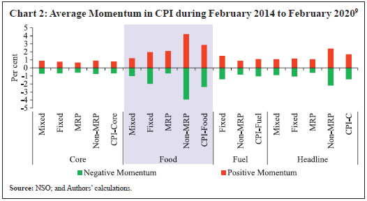 Surprisingly, the only exception to this pattern are the MRP based items in the food group, which show a higher average positive momentum as compared to the average negative momentum, reflecting downward rigidity in the prices of manufactured/packaged food items, which largely belong to the organised retail market. A price rise in the case of a packaged food item owing to certain adverse supply shocks could be easily passed on to the consumers. However, when such adverse shocks wane, the benefits may not be shared with the consumers by lowering product prices or moving back to the pre-shock price levels. This could be possible in food group given their low elasticity of demand as compared with the other household consumption items. Additionally, there is not much visible difference between the average momentum of the four categories in the core group. This is due to the fact that the core group has a high share of services items and most of the items are not subject to the kind of supply shocks that are common in the food group. Further, movements in inflation across the four different pricing-based indices clearly show that inflation in MRP based items has the least fluctuation. Since the formal adoption of flexible inflation targeting (FIT) in India in 2016, inflation in MRP based items has broadly hovered around the medium-term target of 4 per cent, while inflation across the other indices has recorded significant fluctuations on either side of the target (Chart 3). Alternatively, it is found that the distribution of inflation in the case of the MRP based items is strikingly different with much lesser variance, thus, revealing a heavier concentration of inflation around its mean; whereas the rest have much wider and heavier tails indicating the presence of extreme inflation prints (Chart 4). Further, in terms of volatilities of momentum, inflation and change in inflation, the MRP based items exhibit the lowest volatility as compared to the others (Annex Table A2). 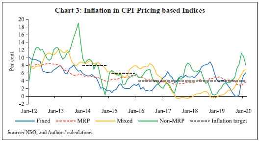 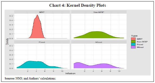 Thus, the above nuances of the CPI-C data indicate that there are some price indices which do not change often and are sticky in nature, while the rest fluctuate more often and are thus, flexible. Therefore, based on these observations, the two sub-indices have been constructed within CPI-C, which are: CPI-sticky price index and CPI-flexible price index. (iii) Sticky and Flexible Price Indices Based on the observed characteristics of the MRP based pricing index, it forms the sticky price index-1 with a share of 19.4 per cent in CPI. Further, considering the fact that the services items within CPI have a lesser frequency of price change along with a lower volatility of inflation and change in inflation10, the CPI-sticky price index-2 is constructed by clubbing together ‘MRP’ and ‘services’, resulting into a combined share of 42.8 per cent in CPI-C. The counterparts of these two indices are termed as the flexible price indices. Table 3 provides the statistical properties of these indices in detail. Table 3: Pricing-based Aggregate Indices in CPI-C – Summary Statistics
(January 2011-February 2020) | | Pricing-based Aggregate Indices | Composition | Momentum11 (per cent) | Inflation (per cent) | Change in Inflation (percentage points) | | Mean | Std. Dev. | Mean | Std. Dev. | Std. Dev. | | Sticky Price Index-1 | MRP (19.4) | 0.42 | 0.23 | 5.03 | 1.58 | 0.28 | | Sticky Price Index-2 | MRP+Services (42.8) | 0.48 | 0.29 | 5.78 | 1.79 | 0.33 | | Flexible Price Index-1 | Fixed+Mixed+Non-MRP (80.6) | 0.49 | 0.79 | 6.08 | 3.13 | 0.92 | | Flexible Price Index-2 | Fixed Goods+Non-MRP Goods+Mixed (57.2) | 0.47 | 1.04 | 5.95 | 3.78 | 1.21 | Note: 1. Figures in parentheses indicate weights in CPI-C.
2. Standard deviation (Std. Dev.) indicates volatility.
Source: NSO; and Authors’ calculations. | It may be observed that the sticky price indices have lower average momentum and inflation as compared to the flexible price indices. Additionally, they also record much lesser volatility in terms of various volatility parameters. Furthermore, it is observed that headline inflation is primarily driven by the movements in the flexible price inflation, while core inflation broadly aligns with the sticky price inflation (Chart 5). Moreover, chart 5 also reveals that while headline inflation eased significantly over the years (up to Q4:2019) in line with a fall in inflation in both sticky and flexible price indices, the extent of easing in core inflation, however, has been relatively less. The observed relative stability in core inflation is largely on account of its composition - a larger share of MRP-based items and services. Accordingly, while average headline inflation moved towards the target of 4 per cent, mean core inflation has stayed higher than the target inflation. Correlation coefficients indicate that inflation in flexible price index-1 has the highest correlation with headline inflation, whereas inflation in sticky price index-2 has the highest correlation with core inflation (Annex Table A3). (iv) Machine Learning Approach to Generate Sticky and Flexible Price Indices: An Alternative Approach As an alternative approach to generate flexible and sticky price indices, a K-means clustering12 is performed on the 299 items of CPI-C. The approach here is to identify two clusters of the items from the basket corresponding to flexible and sticky prices using two key data features - inflation volatility and frequency of price change during January 2014 to February 2020. Items having less inflation volatility and lower frequency of price change are expected to be classified under the sticky price cluster, while items having higher inflation volatility as well as higher frequency of price change are expected to fall under the flexible price cluster.13 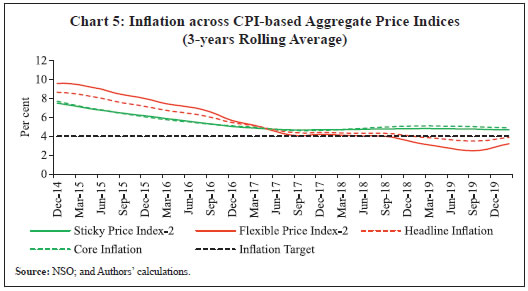 Based on the results of the K-means clustering (K being set to 2), items are classified into sticky and flexible price clusters. These ML-based indices are then compared with pricing-based indices constructed in the previous section. Results show that the two indices move together, thereby providing further credence to our derived pricing-based measures of sticky price indices. In terms of their relationship with headline and core inflation, while headline inflation follows the ML-based flexible price index directionally, magnitude-wise the latter is more volatile (Chart 6a), indicating that the latter is primarily capturing the extreme volatile items of the basket. Further, the sticky price index-2 generated earlier tracks core inflation much better than the ML-based sticky price index (Chart 6b).14 This implies that core inflation is largely influenced by the price movements in the MRP-based items and services.15 Therefore, in the subsequent section, we consider the sticky price index-2 towards estimating the sticky price PC as it largely captures the underlying price movements that are less transient in nature. This implies that any sustained increase in its inflation could indicate building up of persistent price pressures in the economy and therefore, may need constant monitoring. Section IV
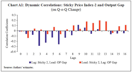
Empirical Evaluation (i) Sticky Price Index and Its Sensitivity to Output Gap Having derived the two sub-indices of CPI-C, in this section we primarily focus on the dynamics of sticky price index. Literature provides ample evidence that sticky prices may not respond to each instance of demand fluctuation and that price stickiness has an impact on output-inflation trade-off (Parkin, 1986; Bryan and Meyer, 2010), which may lead to the non-neutrality of monetary policy (Gali, 2010). Such literature in the Indian context, however, is limited. Therefore, this section studies the linkages between domestic demand conditions/measures of economic slack and the CPI-based sticky price index in a NKPC framework. The sticky-price index-2 is used for this purpose. A cursory look at the data reveals that the sticky price inflation does not have a very close correspondence with the economy-wide measure of slack, which is output gap (Chart 7). Further, pair-wise contemporaneous correlation between quarter-on-quarter (q-o-q) change in sticky price index and output gap turns out to be negative (Annex Table A4). Therefore, dynamic correlations (cross-correlations) are computed to check for any delayed positive association (Annex Chart A1). Results show that changes in sticky price index lag changes in output gap with a significant delay of 2 years and more. Theoretical Framework and Methodology In order to further validate the relationship between sticky price index and demand conditions (proxied by output gap), we base our empirical framework on the insights drawn from the NKPC16 in standard macroeconomic theory. The NKPC, an extension of the original PC with its theoretical micro foundations, has received widespread acceptance in the monetary policy domain and has been widely adopted by central banks globally as the key price determination equation in macro-models. Given this backdrop, a purely forward-looking NKPC resembles equation (1) below: where, πt is inflation at time period t, Et(πt+1) is inflation expectations at time period t and xt represents a proxy for marginal cost or demand conditions17 prevailing in the economy. The disturbance term ut can be interpreted as measurement error or any other combination of unobserved cost-push shocks, such as shocks to the mark-up or input prices (eg., an oil price shock). The principle micro foundation that is inherent in the NKPC framework is the existence of price rigidity, wherein in a microeconomic environment consisting of identical monopolistically competitive firms, firms face constraints on price adjustment18. Literature suggests that even under rational expectations, partial rigidities in the form of information lags or nominal rigidities in prices and wages play a significant role in explaining the observed relationships between inflation and unemployment (Taylor, 1980). Given these facets and empirical difficulties in fitting a purely forward-looking NKPC in the US inflation data, equation (1) underwent modifications that included lagged inflation terms, often termed as ‘intrinsic inflation persistence’ (Mavroeidis et al., 2014). While Gali and Gertler (1999) introduced lagged terms of inflation under the assumption that a fraction of firms updates their prices using some backward-looking rule of thumb, Fuhrer and Moore (1995) relied on the staggered wage contracts to do the same. Some of the newer studies assumed that firms that are unable to re-optimise upon their prices as in the Calvo model often index their prices to past inflation (Christiano et al., 2005; Sbordone, 2005). Thus, the introduction of intrinsic inflation persistence in the PC framework drove the emergence of the ‘hybrid NKPC’, which resembles equation (2) below: 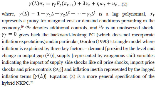 Importantly, the inflation expectations term in equation (2), which is supposed to be an endogenous variable in the system and in fact is unobservable, poses estimation issues in the NKPC framework. Therefore, to correct for such estimation anomalies, literature has come to a consensus on different methods to deal with the inflation expectations variable while estimating the NKPC. These methods include: (i) replacing expectations with actual inflation outcomes and use appropriate instruments (generalised instrumental variables (GIV) framework) [McCallum, 1976; Hansen and Singleton, 1982; Roberts, 1995; Gali and Gertler, 1999]; (ii) deriving expectations in a particular reduced-form model (vector autoregression (VAR) framework) [Fuhrer and Moore, 1995; Sbordone, 2002]; and (iii) using direct measures of expectations (available through inflation expectations surveys) [Roberts, 1995]. Relying on survey-based inflation expectations avoids the need for modelling inflation expectations using statistical/econometric methods, though some researchers feel that the procedure allows for non-rational price setting, the understanding of which is rather limited or at a relatively nascent stage. Therefore, survey-based measures of inflation expectations can be considered as one of the useful ways to look at the intuition behind price-setting being partially forward-looking, partially backward-looking as well as responding to economy-wide aggregate demand conditions. Therefore, considering survey-based inflation expectations in the NKPC framework yields the following representation: 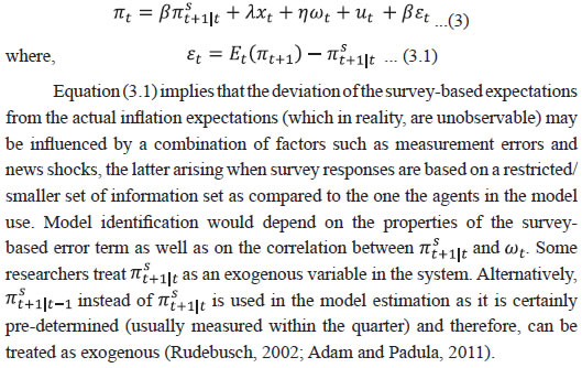 Against this backdrop, equation (4) below forms the base for the empirical framework attempted in this section. (ii) Empirical Estimation and Results Before proceeding for the PC estimation, we first look at the relationship between economic slack (represented by output gap) and the sticky price index-2 and compare that to CPI- C and flexible price index. The slope of the trendline in the case of the sticky price index is flatter as compared to that in the headline CPI-C, while the flexible price index has the steepest slope, indicating its larger reaction to fluctuations in demand conditions in the economy (Chart 8). Therefore, estimation of PC for these indices would enable us to validate this graphical observation. Based on the outlined framework in the previous sub-section [equation (4)], empirical exercise using quarterly data for the sample period 2011:Q1-2019:Q4 is conducted. Data sources used in the empirical exercise are provided in Annex Table A5.1 and variable representation and description are provided in Annex Table A5.2. All variables are converted to their natural logarithms, wherever applicable, and then de-seasonalised using US Census X-13ARIMA method, after which they are used in their first-differenced forms (i.e., q-o-q change) in the model because of their non-stationarity. Stationarity of the variables are tested by employing the augmented Dickey-Fuller (ADF) and Phillips-Perron (PP) tests of unit roots, the results of which are provided in Annex Table A6. 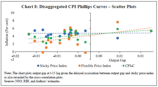 Results presented in table 4 indicate that output gap has a positive and significant impact on the changes in sticky price index and the magnitude of impact turns out to be 0.04 per cent. However, the impact of output gap happens with a significant lag of around 3 years.22 Given the average duration of business cycles to be around five years in India (with an overall range of 2-8 years),23 prices that are sticky may undergo revisions once/twice during such cycles, which could have been possibly reflected in the empirical results obtained. With regard to inflation expectations, results indicate that changes in inflation expectations positively impact sticky price changes with significant lag. The estimated impact turns out to be 0.01 per cent with a lag of 8 quarters.24 The results also point to a significant presence of intrinsic persistence as reflected by the coefficients of the lagged changes in the sticky price index. Having obtained the estimates for the sticky price PC, we now compare the results with the headline PC and the flexible PC estimates (Table 4; columns 2 and 3). The results show that the sticky price PC is much flatter and slower to respond to changes in demand conditions as compared to the headline PC estimates, while the flexible PC is the steepest indicating its larger reaction to fluctuations in demand conditions in the economy, thus, re-validating Chart 8. | Table 4: Regression Results | | | Dependent Variables Δ(In Yi) | | Sticky Price Index | CPI-C | Flexible Price Index | | Explanatory Variables | (1) | (2) | (3) | | Constant | 0.003*
(0.001) | 0.01***
(0.002) | 0.01***
(0.003) | | Δ(In Y)i,t–1 | 0.02
(0.10) | 0.17
(0.11) | 0.23
(0.14) | | Δ(In Y)i,t–3 | 0.36**
(0.09) | 0.37**
(0.15) | - | | Δ(In Y)i,t–12 | 0.21**
(0.05) | - | - | | Δ(one–year ahead inflation expectations)t–j | 0.0001*
(0.0000) | 0.001*
(0.0004) | 0.001*
(0.001) | | (Output Gap)t–k | 0.04**
(0.01) | 0.19*
(0.10) | 0.35*
(0.18) | | No. of Observations | 36 | 36 | 36 | | Sample Period | 2011Q1-2019Q4 | 2011Q1-2019Q4 | 2011Q1-2019Q4 | | Adjusted R-squared | 0.99 | 0.57 | 0.38 | | B-G Serial Correlation LM Test: F-Statistic | 3.51 | 0.21 | 0.66 | | B-P-G Heteroscedasticity Test: F-Statistic | 0.45 | 0.50 | 0.40 | Notes: 1. *, ** and *** represent significance levels at 10 per cent, 5 per cent and 1 per cent, respectively. The variables used in the model were transformed to their natural logarithms and seasonally adjusted before incorporating them in the model. Figures in parentheses indicate heteroscedasticity-consistent standard errors. Δ represents q-o-q change in the variables.
2.Separate period dummies for appropriate quarters were incorporated in the specifications as exogenous variables in order to enhance model performance.
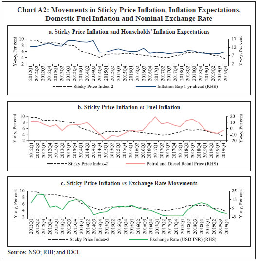
3. The lag structure is as follows: j is 7 in (1), 8 in (2) and 3 in (3); k is 13 in (1) and 6 in (2) and (3). In addition, specification 1 also contains 14th lag of output gap which turned out to be insignificant and specification 2 also consists of 4th lag of dependent variable and 5th lag of output gap. | Overall, the results indicate that the sticky price PC is much flatter as compared to the headline PC followed by the flexible PC, reflecting its meek reaction to changing demand conditions. Additionally, the results also highlight the contribution of intrinsic persistence in imparting price stickiness as indicated by a significantly higher coefficient of its own lags. As a robustness check, another set of regression specification was estimated using control variables such as exchange rate changes, average retail prices of petrol and diesel across four metro cities of India (Kolkata, Delhi, Mumbai and Chennai) as a proxy for input cost pressures, as well as rainfall deviation from the long period average and retail prices of primary vegetables in the case of the flexible price equation. The results (Annex Table A7) are broadly in line with those obtained in Table 4.25 Section V
Conclusion In new Keynesian models, monetary policy can become non-neutral because of the widely observed sticky behaviour in prices. Price stickiness, thus, creates scope for monetary policy to pursue the goals of output and employment. While literature in the Indian context has been devoted largely to validating the presence of the PC and exploring different aspects of inflation forecasting, research on differences in price-setting methods and related heterogeneity in price dynamics at the disaggregated level of the all India CPI has been limited. This paper, therefore, addresses this void in the existing literature and analyses CPI-C at a disaggregated level on the basis of the different price-setting methods. The study first classifies the items based on four different price-setting methods – MRP; non-MRP; a combination of MRP and non-MRP (termed as ‘Mixed’); and Fixed/Regulated – and then using this classification and certain parameters such as ‘price momentum and its volatility’ and ‘inflation and its volatility’ constructs two separate indices, viz., Sticky Price Index and Flexible Price Index. The results show that the sticky price index constitutes around 43 per cent of the overall CPI-C basket and by construction records lower average momentum and inflation as well as much lesser volatility compared to the flexible price index. Furthermore, it is observed that headline inflation is primarily driven by the movements in the flexible price inflation, while core inflation broadly aligns with the sticky price inflation. PC estimates based on the NKPC framework indicate that the sticky price PC is much flatter as compared to the PC based on headline CPI-C and the flexible price PC. Therefore, the results imply that the sticky price PC is less sensitive to changing conditions of economic slack. Additionally, the impact of output gap occurs with a significant lag of around 3 years, suggesting that the sticky price index is slow to adjust to changes in economic slack. Given the average duration of business cycles to be around five years in India, prices that are sticky may undergo revisions once or twice during such cycles, which could possibly be the underlying reason behind the slow and lagged adjustment to output gap. With regard to inflation expectations, results indicate that changes in inflation expectations positively impact sticky price changes, although with some lag. Furthermore, the results reveal a higher degree of intrinsic persistence in the sticky price index, which explains a major part of its stickiness. All of these together imply that in a situation when the sticky price inflation turn upwards, it may remain elevated for a considerable period of time because of its high intrinsic persistence, thus, posing risks for inflation turning generalised. Therefore, monetary policy should remain wary of the underlying inflationary pressures which may be observed by a careful monitoring of the sticky price index. Therefore, from the perspective of India’s monetary policy, analysing movements in the sticky price index could be an important aid in gauging the underlying price pressures in the economy (whether transitory or permanent) and the pricing power of firms, thus providing a deeper understanding of the overall inflation dynamics.
References Adam, K., and Padula, M. (2011). Inflation dynamics and subjective expectations in the United States. Economic Inquiry, 49(1), 13-25. Álvarez, L. J., Burriel, P., and Hernando, I. (2010). Price-setting behaviour in Spain: Evidence from micro PPI data. Managerial and Decision Economics, 31(2-3), 105-121. Alvarez, L. J., Dhyne, E., Hoeberichts, M. M., Kwapil, C., Bihan, L. H., Lunnemann, P., Martins, F., Sabbatini, R., Stahi, H., Vermeulen, P. and Vilumnen, J. (2006). Sticky prices in the euro area: a summary of new micro-evidence. Journal of the European Economic Association, 4(2/3), 575-584 Aucremanne, L., and Dhyne, E. (2004). How frequently do prices change? Evidence based on the micro data underlying the Belgian CPI. European Central Bank Working Paper No. 331, April. Ball, L. and Romer, D. H. (1987). Sticky prices as coordination failure. National Bureau of Economic Research, Working Paper No. w2327. Banerjee, S. and R. Bhattacharya (2017). Micro-level price setting behaviour in India: evidence from group and sub-group level CPI-IW data. NIPFP Working paper No. 217. Banerjee, S., Basu, P., and Ghate, C. (2020). A monetary business cycle model for India. Economic Inquiry, 58(3), 1362-1386. Baudry, L., Bihan H. L., Sevestre, P. and S. Tarrieu (2004). Price rigidity- Evidence from French CPI micro-data. European Central Bank, Working Papers Series No 384, August. Baumgartner, J., Glatzer, E., Rumler, F. and Stiglbauer, A. (2005). How frequently do consumer prices change in Austria? Evidence from micro CPI data. European Central Bank, Working Paper Series No. 523, September. Behera, H. K., and Patra, M. D. (2020). Measuring trend inflation in India”, RBI Working Paper Series: 15/2020. Behera, H. K., Wahi, G., and Kapur, M. (2017). Phillips curve relationship in India: Evidence from state level analysis. RBI Working Paper Series : 08/2017. Behera, H. and Sharma, S. (2019). Does financial cycle exist in India?. RBI Working Paper Series: 03/2019 Bils, M, P. Klenow and O. Kryvtsov (2003). Sticky prices and monetary policy shocks. Federal Reserve Bank of Minneapolis, Quarterly Review,27(1), Winter 2003, pp. 2–9 Bils, M., and Klenow, P. J. (2004). Some evidence on the importance of sticky prices. Journal of political economy, 112(5), 947-985. Blanchard, O.J. (1983). Price asynchronization and price level inertia, in inflation, debt and indexation. R. Dornbusch and M. Simonsen eds., Inflation, Debt and Indexation, MIT Press, pp. 3—24. Blinder, A. S. (1993). Why are prices sticky? Preliminary results from an interview study. In Optimal Pricing, Inflation and the Cost of Price Adjustment, Eytan S. and Yoram, W. eds. MIT Press, Cambridge, MA (pp. 409-421). Blinder, A.S. (1982). Inventories and sticky prices: More on the microfoundations of macroeconomics. American Economic Review, 72(3), June, pp. 334-348. Boivin J., Giannoni, M.P., and Mihov, I. (2009). Sticky prices and monetary policy: Evidence from disaggregated US data. American Economic Review, 99(1), March, pp. 350–384. Bryan, M. F. and Meyer, B. (2010). Are some prices in the CPI more forward looking than others? We think so. Federal Reserve of Cleveland, Economic Commentary Number 2010-2, May 19, 2010. Caballero, R. J. and Engel, E. M.R.A. (2006). Price stickiness in Ss models: Basic properties”, MIT. Calvo, G. A. (1983). Staggered prices in a utility-maximizing framework. Journal of Monetary Economics, 12(3), 383-398. Cecchetti, S. G. (1986). The frequency of price adjustment: A study of the newsstand prices of magazines. Journal of Econometrics, 31(3), 255-274. Chong, T.T.L., Rafiq, M.S., and Zhu, T. (2013). Are prices sticky in large developing economies? An empirical comparison of China and India. MPRA Paper No. 60985, December 2013. Christiano, L. J., Eichenbaum, M., and Evans, C. L. (2005). Nominal rigidities and the dynamic effects of a shock to monetary policy. Journal of Political Economy, 113(1), 1-45. Cooper, R., and John, A. (1988). Coordinating coordination failures in Keynesian models. The Quarterly Journal of Economics, 103(3), 441-463. Dholakia, R. H., and Kandiyala, V. S. (2018). Changing dynamics of inflation in India”, Economic and Political Weekly, 53(9), 65-73. Dhyne, E., Alvarez, L. J., Bihan, L.H., Veronese, G., Dias, D., Hoffmann, J, Jonker, N., Lunnemann, P., Rumler, F. and Vilmunen, J. (2005). Price setting in the euro area: Some stylized facts from individual consumer price data. European Central Bank, Working Paper Series No. 524, September. Dias, M., Dias, D., and Neves, P. D. (2004). Stylised features of price setting behaviour in Portugal: 1992-2001. European Central Bank, Working Paper Series No. 332. Dotsey, M., King, R. G., and Wolman, A. L. (1999). State-dependent pricing and the general equilibrium dynamics of money and output. The Quarterly Journal of Economics, 114(2), 655-690. Erceg, C. J., Henderson, D. W., and Levin, A. T. (2000). Optimal monetary policy with staggered wage and price contracts. Journal of Monetary Economics, 46(2), 281-313. Erlandsen, S.K. (2014). Sticky prices and inflation expectations in Norway. Staff Memo No. 14, 2014, Norges Bank. Fischer, S. (1977). Long-term contracts, rational expectations, and the optimal money supply rule. Journal of Political Economy, 85(1), 191-205. Fisher, P. G., Mahadeva, L., & Whitley., J. D. (1997). The output gap and inflation–experience at the Bank of England. BIS Conference Papers, Vol. 4. Fougère, D., Bihan, H. L., and Sevestre, P. (2005). Heterogeneity in price stickiness: a microeconometric investigation.European Central Bank, Working Paper Series No. 536, October. Fuhrer, J., and Moore, G. (1995). Inflation persistence. The Quarterly Journal of Economics, 110(1), 127-159. Gagnon, E., and Khan, H. (2001). New Phillips curve with alternative marginal cost measures for Canada, the United States, and the Euro Area. Bank of Canada (No. 2001-25). Gali, J., and Gertler, M. (1999). Inflation dynamics: A structural econometric analysis. Journal of Monetary Economics, 44(2), 195-222. Gali, J., Gertler, M., and Lopez-Salido, J. D. (2001). European inflation dynamics. European Economic Review, 45(7), 1237-1270. Galí, J. (2010). The New-Keynesian approach to monetary policy analysis: Lessons and new directions. In The science and practice of monetary policy today, pp. 9-19. Springer, Berlin, Heidelberg. Ghani, E. (1991). Rational expectations and price behavior: A study of India. Journal of Development Economics, 36 (2), October, pp. 295-311. Gordon, R. J. (1981). Output fluctuations and gradual price adjustment. National Bureau of Economic Research, Working Paper Series, w0621. Hall, R. E., Blanchard, O. J., and Hubbard, R. G. (1986). Market structure and macroeconomic fluctuations. Brookings papers on economic activity, 1986(2), 285-338. Hansen, L. P., and Singleton, K. J. (1982). Generalized instrumental variables estimation of nonlinear rational expectations models. Econometrica: Journal of the Econometric Society, 50(5), September, pp. 1269-1286. Henkel, L. (2020). Sectoral output effects of monetary policy: Do sticky prices matter? European Central Bank, Working Paper Series No. 2473, October. John, J., Singh, S. and Kapur, M. (2020). Inflation forecast combinations – The Indian experience”, RBI Working Paper Series : 11/2020. Jose, J., Shekhar, H., Kundu S., Kishore, V. and Bhoi B. B. (2022). Alternative inflation forecasting models for India –What performs better in practice?”, RBI Occasional Papers, Vol. 42(1). Kashyap, A.K. (1995). Sticky prices: New evidence from retail catalogs. The Quarterly Journal of Economics, 110 (1), February, pp. 245-274. Kiley, M.T., (2000). Endogenous price stickiness and business cycle persistence. Journal of Money, Credit and Banking, February, 2000, 32(1), pp. 28-53. Knotek II, E. S. (2010). A tale of two rigidities: Sticky prices in a sticky-information environment. Journal of Money, Credit and Banking, 42(8), 1543-1564. Mankiw, N. G. (1985). Small menu costs and large business cycles: A macroeconomic model of monopoly. The Quarterly Journal of Economics, 100(2), 529-537. Mankiw, N. G., and Reis, R. (2002). Sticky information versus sticky prices: a proposal to replace the New Keynesian Phillips curve. The Quarterly Journal of Economics, 117(4), 1295-1328. Mavroeidis, S., Plagborg-Møller, M., and Stock, J. H. (2014). Empirical evidence on inflation expectations in the New Keynesian Phillips Curve. Journal of Economic Literature, 52(1), 124-88. Mazumder, S. (2011). The empirical validity of the New Keynesian Phillips curve using survey forecasts of inflation. Economic Modelling, 28(6), 2439-2450. McCallum, B. T. (1976). Rational expectations and the natural rate hypothesis: some consistent estimates. Econometrica. Journal of the Econometric Society, 44(1), January, pp. 43-52. Millard, S. and O’Grady, T. (2012). What do sticky and flexible prices tell us?”, Bank of England Working Paper No. 457, July 20. 2012. Nadhanael, G.V. (2020). Are food prices really flexible? Evidence from India. RBI Working Paper Series: 10/2020. Nakamura, E., and Steinsson, J. (2010). Monetary non-neutrality in a multisector menu cost model. The Quarterly Journal of Economics, 125(3), 961-1013. National Sample Survey Office (NSSO). (2014). Household consumption of various goods and services in India 2011-12. Government of India, June 2014. Parkin, M. (1986). The output-inflation trade-off when prices are costly to change. Journal of Political Economy, 94 (1), February, pp. 200-224. Patra, M.D., Behera, H. and John, J. (2021). Is the Phillips Curve in India Dead, Inert and Stirring to Life or Alive and Well? RBI Bulletin Article, November 2021. Pratap, B., and Sengupta, S. (2019). Macroeconomic forecasting in India: Does machine learning hold the key to better forecasts? RBI Working Paper Series: 04/2019. Rangarajan, C., Dev, S. M., Sundaram, K., Vyas, M. and Datta, K.L., (2014). Report of the expert group to review the methodology for measurement of poverty. Planning Commission, June 2014 Rather, S.R., Durai, S.R.S. and Ramachandran, M. (2015). Asymmetric price adjustment – evidence for India. The Journal of Economic Asymmetries, 12 (2), November, pp. 73-79. Reiff, A. and Varhegyi, J. (2013). Sticky price inflation index: An alternative core inflation measure. MNB Working Papers, No. 2013/2, Magyar Nemzeti Bank, Budapest. Roberts, J. M. (1995). New Keynesian economics and the Phillips curve. Journal of Money, Credit and Banking, 27(4), 975-984. Rotemberg, J. J. (1982). Sticky prices in the United States. Journal of Political Economy, 90(6), pp. 1187-1211. Rudebusch, G. D. (2002). Assessing nominal income rules for monetary policy with model and data uncertainty. The Economic Journal, 112(479), pp. 402-432. Sbordone, A. M. (2002). Prices and unit labor costs: a new test of price stickiness. Journal of Monetary Economics, 49(2), pp. 265-292. Sbordone, A. M. (2005). Do expected future marginal costs drive inflation dynamics? Journal of Monetary Economics, 52(6), pp. 1183-1197. Taylor, J. B. (1979). Staggered wage setting in a macro model. The American Economic Review, 69(2), pp. 108-113. Taylor, J. B. (1980). Aggregate dynamics and staggered contracts. Journal of political economy, 88(1), pp. 1-23. Tripathi, S. and Goyal, A. (2012). Relative prices, the price level and inflation: Effects of asymmetric and sticky adjustment. IGIDR, WP-2011-026. Vilmunen, J. and H. Laakkonen (2005). How often do prices change in Finland? Evidence from micro CPI data. Bank of Finland, unpublished mimeo. Zbaracki, M. J., Ritson, M., Levy, D., Dutta, S., and Bergen, M. (2004). Managerial and customer costs of price adjustment: direct evidence from industrial markets. Review of Economics and statistics, 86(2), pp. 514-533.
Annex | Table A1: Classification of Items | | S. No | MRP | Non-MRP | Mixed | Fixed | | 1 | medicine [non-institutional] (4) | house rent; garage rent (9.5) | milk: liquid (litre) (6.4) | tuition and other fees [school; college; etc.] (2.9) | | 2 | mustard oil (1.3) | cooked meals purchased (no.) (2.4) | rice_other sources (4.4) | electricity (std. unit) (2.3) | | 3 | refined oil [sunflower; soyabean; saffola; etc.] (1.3) | firewood and chips (2.1) | wheat/atta_other sources (2.6) | petrol for vehicle (2.2) | | 4 | tea: leaf (gm) (1) | fish; prawn (1.3) | sugar - other sources (1.1) | telephone charges: mobile (1.8) | | 5 | biscuits; chocolates; etc. (0.9) | chicken (1.2) | arhar; tur (0.8) | bus/tram fare (1.4) | | 6 | washing soap/soda/powder (0.9) | cooked snacks purchased [samosa; puri; paratha; burger; chowmein; idli; dosa; vada; chops; pakoras; pao bhaji; etc.] (1.2) | dry chillies (gm) (0.6) | LPG [excl. conveyance] (1.3) | | 7 | motor cycle; scooter (0.8) | gold (1.1) | turmeric (gm) (0.5) | taxi; auto-rickshaw fare (0.6) | | 8 | toilet soap (0.6) | potato (1) | ghee (0.5) | rice_PDS (0.4) | | 9 | books; journals: first hand (0.6) | saree (no.) (0.9) | jeera (gm) (0.4) | kerosene PDS (litre) (0.3) | | 10 | motor car; jeep (0.5) | tea: cups (no.) (0.9) | moong (0.3) | school bus; van; etc. (0.2) | | 11 | papad; bhujia; namkeen; mixture; chanachur (0.5) | monthly charges for cable TV connection (0.8) | dhania (gm) (0.3) | railway fare (0.2) | | 12 | hair oil; shampoo; hair cream (0.5) | goat meat/mutton (0.8) | masur (0.3) | wheat/atta_PDS (0.2) | | 13 | bidi (no.) (0.4) | doctors/surgeons fee- first consultation [non-institutional] (0.8) | urd (0.3) | telephone charges: landline (0.2) | | 14 | foreign/refined liquor or wine (litre) (0.4) | cloth for shirt; pyjama; kurta; salwar; etc. (metre) (0.7) | leather boots; shoes (0.2) | water charges (0.2) | | 15 | powder; snow; cream; lotion and perfume (0.4) | onion (0.6) | gram: split (0.2) | diesel for vehicle (0.1) | | 16 | toothpaste; toothbrush; comb; etc. (0.4) | domestic servant/cook (0.6) | leather sandals; chappals; etc. (0.2) | sugar - PDS (0.1) | | 17 | country liquor (litre) (0.4) | private tutor/coaching centre (0.6) | gamchha; towel; handkerchief (no.) (0.2) | diesel (litre) [excl. conveyance] (0) | | 18 | groundnut oil (0.3) | tomato (0.6) | other petty articles (0.2) | - | | 19 | rubber/PVC footwear (0.3) | shirts; T-shirts (no.) (0.6) | besan (0.2) | - | | 20 | cigarettes (no.) (0.2) | other vegetables (0.6) | tamarind (gm) (0.1) | - | | 21 | incense [agarbatti]; room freshener (0.2) | banana (no.) (0.6) | black pepper (gm) (0.1) | - | | 22 | bed sheet; bed cover (no.) (0.2) | prepared sweets; cake; pastry (0.6) | other washing requisites (0.1) | - | | 23 | electric bulb; tubelight (0.2) | shorts; trousers; bermudas (no.) (0.6) | chira (0.1) | - | | 24 | newspapers; periodicals (0.2) | barber; beautician; etc. (0.6) | gram: whole (0.1) | - | | 25 | curry powder (gm) (0.2) | baniyan; socks; other hosiery and undergarments; etc. (no.) (0.5) | curd (0.1) | - | | 26 | television (0.2) | X-ray; ECG; pathological test; etc. [non-institutional] (0.5) | oilseeds (gm) (0.1) | - | | 27 | salt (0.2) | apple (0.5) | cashewnut (0.1) | - | | 28 | mobile handset (0.1) | dung cake (0.4) | other leather footwear (0.1) | - | | 29 | bicycle [without accessories] (0.1) | hospital and nursing home charges (0.4) | peas [Pulses] (0.1) | - | | 30 | mosquito repellent; insecticide; acid etc. (0.1) | palak/other leafy vegetables (0.4) | bucket; water bottle/feeding bottle and other plastic goods (0.1) | - | | 31 | sports goods; toys; etc. (0.1) | eggs (no.) (0.4) | maize and products (0.1) | - | | 32 | PC/Laptop/other peripherals incl. software (0.1) | cloth for coat; trousers; suit; etc. (metre) (0.4) | raisin; kishmish; monacca; etc. (0.1) | - | | 33 | bread [bakery] (0.1) | tailor (0.4) | cereal substitutes: tapioca; etc. (0) | - | | 34 | shaving blades; shaving stick; razor (0.1) | stationery; photocopying charges (0.4) | other dry fruits (0) | - | | 35 | suji; rawa (0.1) | brinjal (0.4) | ragi and its products (0) | - | | 36 | pickles (gm) (0.1) | grinding charges (0.3) | dates (0) | - | | 37 | refrigerator (0.1) | mango (0.3) | almirah; dressing table (0) | - | | 38 | sanitary napkins (0.1) | garlic (gm) (0.3) | maida (0) | - | | 39 | cold beverages: bottled/canned (litre) (0.1) | groundnut (0.3) | other furniture and fixtures [couch; sofa; etc.] (0) | - | | 40 | other beverages: cocoa; chocolate; etc. (0.1) | residential building and land [cost of repairs only] (0.3) | gram products (0) | - | | 41 | matches (box) (0.1) | ladys finger (0.3) | other rice products (0) | - | | 42 | coconut oil (0.1) | green chillies (0.3) | chair; stool; bench; table (0) | - | | 43 | other packaged processed food (0.1) | beef/buffalo meat (0.3) | other metal utensils (0) | - | | 44 | rug; blanket (no.) (0.1) | other tobacco products (0.3) | other crockery and utensils (0) | - | | 45 | tyres and tubes (0.1) | coconut (no.) (0.3) | headwear; belts; ties (no.) (0) | - | | 46 | vanaspati; margarine (0.1) | cauliflower (0.2) | coir; rope; etc. (0) | - | | 47 | umbrella; raincoat (0.1) | gourd; pumpkin (0.2) | walnut (0) | - | | 48 | beer (litre) (0.1) | jowar and its products (0.2) | cloth for upholstery; curtains; tablecloth; etc. (metre) (0) | - | | 49 | coffee: powder (gm) (0.1) | kurta-pajama suits: females (no.) (0.2) | goods for recreation and hobbies (0) | - | | 50 | air conditioner; air cooler (0.1) | kerosene other sources (litre) (0.2) | carpet; daree and other floor mattings (0) | - | | 51 | fruit juice and shake (litre) (0.1) | coat; jacket; sweater; windcheater (no.) (0.2) | glassware (0) | - | | 52 | lubricants and other fuels for vehicle (0.1) | ginger (gm) (0.2) | candy; misri (0) | - | | 53 | zarda; kimam; surti (gm) (0) | other fuel (0.2) | other cereals (0) | - | | 54 | pillow; quilt; mattress (no.) (0) | cabbage (0.2) | bedding: others (0) | - | | 55 | torch (0) | stainless steel utensils (0.2) | knitting wool (gm) (0) | - | | 56 | shaving cream; aftershave lotion (0) | other footwear (0.2) | small millets and their products (0) | - | | 57 | inverter (0) | school/college uniform: boys (0.2) | any other personal goods (0) | - | | 58 | milk: condensed/ powder (0) | other consumer services excluding conveyance (0.2) | - | - | | 59 | sewai; noodles (0) | pan: finished (no.) (0.2) | - | - | | 60 | candle (no.) (0) | grapes (0.2) | - | - | | 61 | baby food (0) | frocks; skirts; etc. (no.) (0.2) | - | - | | 62 | washing machine (0) | beans; barbati (0.1) | - | - | | 63 | sauce; jam; jelly (gm) (0) | school/college uniform: girls (0.1) | - | - | | 64 | mineral water (litre) (0) | ingredients for pan (gm) (0.1) | - | - | | 65 | electric fan (0) | cinema: new release [normal day] (0.1) | - | - | | 66 | mosquito net (no.) (0) | lemon (no.) (0.1) | - | - | | 67 | ice-cream (0) | orange; mausami (no.) (0.1) | - | - | | 68 | electric batteries (0) | washerman; laundry; ironing (0.1) | - | - | | 69 | butter (0) | other fresh fruits (0.1) | - | - | | 70 | water purifier (0) | other medical expenses [non-institutional] (0.1) | - | - | | 71 | chips (gm) (0) | watch man charges [other cons taxes] (0.1) | - | - | | 72 | VCR/VCD/DVD player (0) | lungi (no.) (0.1) | - | - | | 73 | other cooking/household appliances (0) | other entertainment (0.1) | - | - | | 74 | CD; DVD; audio/video cassette; etc. (0) | bajra and its products (0.1) | - | - | | 75 | other durables [specify] (0) | silver (0.1) | - | - | | 76 | plugs; switches and other electrical fittings (0) | muri (0.1) | - | - | | 77 | radio; tape recorder; 2-in-1 (0) | peas [Vegetables] (0.1) | - | - | | 78 | honey (0) | gur (0.1) | - | - | | 79 | camera and photographic equipment (0) | coconut: copra (0.1) | - | - | | 80 | electric iron; heater; toaster; oven and other electric heating appliances (0) | leaf tobacco (gm) (0.1) | - | - | | 81 | bathroom and sanitary equipment (0) | parwal/patal; kundru (0.1) | - | - | | 82 | suitcase; trunk; box; handbag and other travel goods (0) | carrot (0.1) | - | - | | 83 | lock (0) | flower [fresh]: all purposes (0.1) | - | - | | 84 | sewing machine (0) | other pulses (0.1) | - | - | | 85 | lighter [bidi/cigarette/gas stove] (0) | shawl; chaddar (no.) (0.1) | - | - | | 86 | pressure cooker/pressure pan (0) | guava (0.1) | - | - | | 87 | family planning devices (0) | internet expenses (0.1) | - | - | | 88 | clock; watch (0) | air fare [normal]: economy class [adult] (0.1) | - | - | | 89 | stove; gas burner (0) | other intoxicants (0.1) | - | - | | 90 | - | dhoti (no.) (0.1) | - | - | | 91 | - | radish (0.1) | - | - | | 92 | - | pan: leaf (no.) (0.1) | - | - | | 93 | - | toddy (litre) (0.1) | - | - | | 94 | - | bedstead (0.1) | - | - | | 95 | - | spectacles (0.1) | - | - | | 96 | - | kurta-pajama suits: males (no.) (0.1) | - | - | | 97 | - | pork (0.1) | - | - | | 98 | - | clothing [first-hand]: other (0.1) | - | - | | 99 | - | papaya (0) | - | - | | 100 | - | watermelon (0) | - | - | | 101 | - | green coconut (no.) (0) | - | - | | 102 | - | rickshaw [hand drawn and cycle] fare (0) | - | - | | 103 | - | sweeper (0) | - | - | | 104 | - | other educational expenses [incl. fees for enrollment in web-based training] (0) | - | - | | 105 | - | Monthly Maintainance charges (0) | - | - | | 106 | - | coal (0) | - | - | | 107 | - | other pulse products (0) | - | - | | 108 | - | earthenware (0) | - | - | | 109 | - | other milk products (0) | - | - | | 110 | - | photography (0) | - | - | | 111 | - | coffee: cups (no.) (0) | - | - | | 112 | - | other nuts (0) | - | - | | 113 | - | clothing: second-hand (0) | - | - | | 114 | - | kharbooza (0) | - | - | | 115 | - | other ornaments (0) | - | - | | 116 | - | khesari (0) | - | - | | 117 | - | coke (0) | - | - | | 118 | - | other conveyance expenses (0) | - | - | | 119 | - | hotel lodging charges (0) | - | - | | 120 | - | leechi (0) | - | - | | 121 | - | hookah tobacco (gm) (0) | - | - | | 122 | - | others: birds; crab; oyster; tortoise; etc. (0) | - | - | | 123 | - | cheroot (no.) (0) | - | - | | 124 | - | jackfruit (0) | - | - | | 125 | - | horse cart fare (0) | - | - | | 126 | - | pineapple (no.) (0) | - | - | | 127 | - | VCD/DVD hire [incl. instrument] (0) | - | - | | 128 | - | charcoal (0) | - | - | | 129 | - | singara (0) | - | - | | 130 | - | porter charges (0) | - | - | | 131 | - | club fees (0) | - | - | | 132 | - | berries (0) | - | - | | 133 | - | snuff (gm) (0) | - | - | | 134 | - | pears/nashpati (0) | - | - | | 135 | - | steamer; boat fare (0) | - | - | | 136 | - | library charges (0) | - | - | | Items | 89 | 136 | 57 | 17 | | Weight | 19.4 | 45.2 | 21.1 | 14.3 |
| Table A2: Volatility (Standard Deviation: January 2011 to February 2020) | | Price Indices | Momentum | Inflation | Change in Inflation | | MRP | 0.2 | 1.6 | 0.3 | | Non-MRP | 1.2 | 3.9 | 1.5 | | Mixed | 0.5 | 3.8 | 0.6 | | Fixed | 0.6 | 2.5 | 0.8 | | Source: NSO; and Authors’ calculations. |
| Table A3: Correlation between Headline/Core Inflation and Inflation in Sticky and Flexible Price Indices | | Indices | Headline Inflation | Core Inflation | | Sticky price index-1 | 0.76*** | 0.90*** | | Flexible price index-1 | 0.99*** | 0.72*** | | Sticky price index-2 | 0.81*** | 0.95*** | | Flexible price index-2 | 0.97*** | 0.63*** | | Sticky price index-ML | 0.92*** | 0.89*** | | Flexible price index-ML | 0.75*** | 0.28*** | | Headline Inflation | 1.00*** | 0.77*** | Note: Coefficients are significant at 1 per cent level of significance.
Source: NSO; and Authors’ calculations. |
| Table A4: Contemporaneous Correlation Coefficients (on Q-o-Q change) | | Variables | Sticky Price Index 1 | Sticky Price Index 2 | | Sticky Price Index-1 | 1.00 | 0.88*** | | Sticky Price Index-2 | 0.88*** | 1.00 | | Flexible Price Index-1 | 0.42** | 0.64*** | | Flexible Price Index-2 | 0.35** | 0.56*** | | Inflation Expectations (1 year ahead) | 0.51*** | 0.50*** | | Inflation Expectations (3 months ahead) | 0.45*** | 0.46*** | | Output Gap | -0.34** | -0.26 | | Petrol and Diesel Retail Prices | 0.15 | 0.22 | | Global Non-Fuel Price | -0.26 | -0.28 | | Exchange Rate (INR-USD) | 0.38** | 0.40** | | Note: ***, ** and * indicate significance at 1 per cent, 5 per cent and 10 per cent levels of significance, respectively. |
| Table A5.1: Data Sources | | S. No. | Variables | Source | | 1. | CPI-C | National Statistical Office (NSO), Ministry of Statistics and Programme Implementation (MOSPI), GoI | | 2. | INR-USD Exchange Rate | Database on Indian Economy (DBIE), RBI | | 3. | Petrol and Diesel Retail Prices | Indian Oil Corporation Limited (IOCL) | | 4. | Global Non-fuel Price Indices | World Bank Pink Sheet Database | | 5. | Rainfall Deviation from LPA | India Meteorological Department (IMD) | | 6. | Inflation Expectations | Inflation Expectations Survey of Households (IESH), RBI | | 7. | Real Gross Domestic Price (GDP) [Base year: 2011-12=100] | NSO, MoSPI, GoI | | 8. | Tomato-Onion-Potato (TOP) prices | Department of Consumer Affairs (DCA), Ministry of Consumer Affairs, Food and Public Distribution, GoI | | 9. | Rural Wages | Labour Bureau, Ministry of Labour and Employment, GoI |
| Table A5.2: Variable Description and Representation | | S. No. | Variables | Representation | | 1. | CPI-C and other derived indices | Y | | 2. | INR-USD Exchange Rate | Nominal exchange rate | | 3. | Petrol and Diesel Retail Prices: average retail prices of petrol and diesel across four metro cities of India (Kolkata, Delhi, Mumbai and Chennai) | RetailPrice_Petrol&Diesel | | 4. | Rainfall Deviation from the long period average (LPA) | Rain Dev from LPA | | 5. | Inflation Expectations | One-year ahead households’ inflation expectations | | 6. | Output Gap: Calculated as log of actual seasonally adjusted real GDP series less its Hodrick-Prescott filtered trend*100. | Output Gap | | 7. | Tomato-Onion-Potato (TOP) prices: Average of retail prices | DCA TOP |
| Table A6: Unit Root Test Results | | De-seasonalised Variables | ADF Test | PP Test | | log(x) | Δ log(x) | log(x) | Δ log(x) | | Sticky Price Index-1 | -3.50* | -3.65** | -3.22* | -3.65** | | Sticky Price Index-2 | -4.09** | -3.69** | -3.64** | -3.83** | | Output Gap# | -7.45*** | -9.53*** | - | - | | Exchange Rate (INR-USD) | -2.67 | -5.84*** | -1.87 | -6.50*** | | Global Non-fuel Prices | -1.2 | -4.56*** | -0.56 | -4.58*** | | Domestic Petrol and Diesel Prices | -2.12 | -2.44 | -2.24 | -5.46*** | | DCA TOP Prices | -2.91 | -6.74*** | -3.29* | -6.79*** | | Rural Wage | -3.81** | -5.61*** | -2.31 | -3.81** | | Non-De-seasonalised Variable | x | Δx | x | Δx | | Rainfall Deviation from LPA | -5.14*** | -6.40*** | -5.13*** | -14.96*** | | Inflation Expectations (1year ahead) | -3.2 | -6.60*** | -3.23* | -7.88*** | | Note: ***, ** and * indicate significance at 1 per cent, 5 per cent and 10 per cent levels of significance, respectively. #: tested for structural break unit root test. |
| Table A7: Regression Results - With Controls | | Explanatory Variables | Dependent Variables Δ(In Yi) | | Sticky Price Index (1) | CPI-C (2) | Flexible Price Index (3) | | Constant | 0.0004
(0.001) | 0.005**
(0.002) | 0.007***
(0.002) | | Δ(In Y)i,t–1 | 0.10**
(0.03) | 0.38***
(0.12) | - | | Δ(In Y)i,t–2 | - | - | 0.15*
(0.08) | | Δ(In Y)i,t–3 | 0.10***
(0.02) | - | - | | Δ(In Y)i,t–12 | 0.34***
(0.02) | - | - | | Δ(one–year ahead inflation expectations)t–i | 0.0003***
(0.0000) | 0.001*
(0.0003) | 0.0002
(0.0003) | | Δ(In RetailPrice_Petrol&Diesel)t–j | 0.03***
(0.002) | 0.05**
(0.02) | 0.003
(0.02) | | (Output Gap)t–k | 0.08***
(0.01) | 0.21*
(0.10) | 0.26**
(0.10) | [Dummy_Output Gap*
Δ(In RetailPrice_Petrol&Diesel)t–l | 0.08***
(0.002) | - | 0.06
(0.05) | | Δ(In Exchange rate)t–m | 0.07***
(0.005) | 0.10**
(0.0003) | 0.10***
(0.02) | | (Rain Dev from LPA)t–3 | - | - | 0.0002***
(0.0000) | | Δ(In DCATOP)t | - | - | 0.06***
(0.01) | | No. of Observations | 36 | 36 | 36 | | Sample Period | 2011Q1-2019Q4 | 2011Q1-2019Q4 | 2011Q1-2019Q4 | | Adjusted R-squared | 0.95 | 0.48 | 0.82 | | B-G Serial Correlation LM Test: F-Statistic | 0.91 | 0.71 | 2.10 | | B-P-G Heteroscedasticity Test: F-Statistic | 0.92 | 0.76 | 1.10 | Notes: 1. *, ** and *** represent significance levels at 10 per cent, 5 per cent and 1 per cent, respectively. The variables used in the model were transformed to their natural logarithms and seasonally adjusted before incorporating them in the model. Figures in parentheses indicate heteroscedasticity-consistent standard errors. ∆ represents q-o-q change in the variables.
2. Separate period dummies for appropriate quarters were incorporated in the specifications as exogenous variables in order to enhance model performance.
3. The lag structure is as follows: i is 8 in (1) and (2) and 1 in (3); j is 2 in (1), 7 in (2) and 5 in (3); k is 13 in (1), 6 in (2) and 7 in (3); l is 5 in (1) and 0 in (3); m is 1 in (1), 5 in (2) and 7 in (3); n1 is 0 in (1), 2 in (2) and 0 in (3). Other controls used were other lags of output gap, respective dependent variables and change in rural wages. |
|