2.1 Scheduled Commercial Banks (a) Banking stability indicator The banking stability indicator presents an overall assessment of changes in underlying conditions and risk factors that have a bearing on the stability of the banking sector during a period. The six composite indices represent risk in six dimensions - soundness, asset quality, profitability, liquidity, efficiency and sensitivity to market risk. Each composite index is a relative measure of risk during the sample period used for its construction, where a higher value would mean higher risk in that dimension. The financial ratios used for constructing each composite index are given in Table 1. Each financial ratio is first normalised for the sample period using the following formula: where Xt is the value of the ratio at time t. If a variable is negatively related to risk, then normalisation is done using 1-Yt. Composite index of each dimension is then calculated as a simple average of the normalised ratios in that dimension. Finally, the banking stability indicator is constructed as a simple average of these six composite indices. Thus, each composite index and the overall banking stability indicator take values between zero and one. | Table 1: Ratios used for constructing the banking stability indicator | | Dimension | Ratios | | Soundness | CRAR # | Nonperforming Loans net of Provisions-to-Capital | Tier 1 Capital-to-Assets # | | | Asset Quality | Gross NPAs-to-Total Advances | Provisions-to-Nonperforming Loans # | Sub-standard Advances-to-Gross NPAs # | Restructured Standard Advances-to-Standard Advances | | Profitability | Return on Assets # | Net Interest Margin # | Growth in Profit before Tax # | Interest Margin-to-Gross Income # | | Liquidity | Liquid Assets-to-Total Assets # | Liquidity Coverage Ratio # | Customer Deposits-to-Total Assets # | Non-Bank Advances-to-Customer Deposits | | Efficiency | Cost-to-Income | Business (Credit + Deposits)-to-Staff Expenses # | Staff Expenses-to-Total Expenses | | | Sensitivity to market risk | RWA (market risk)-to-Capital | Trading Income-to-Gross Income | | | | Note: # Negatively related to risk. | (b) Macro stress testing Macro stress test ascertains the resilience of banks against macroeconomic shocks by assessing the impact of macro shocks on capital adequacy of a set of major scheduled commercial banks (46 banks presently). Macro stress test attempts to project capital ratios over a one-year horizon, under a baseline and two adverse (medium and severe) scenarios. The macro stress test framework consists of (i) designing the macro scenarios, (ii) projection of GNPA ratios, (iii) projection of profit after tax (PAT), (iv) projection of sectoral probability of default (PD) and (v) projection of capital ratios. I. Designing Macro Scenarios II. Projection of GNPA ratios GNPA ratios are projected for each of the three bank groups, viz, public sector banks (PSBs), private sector banks (PVBs) and foreign banks (FBs). Natural logarithm of GNPA ratios of these bank-groups are modelled using two complementary econometric models, viz; (i) Autoregressive distributed lag (ADL) model and (ii) Vector auto regression (VAR) model. The values projected based on both these models are averaged to arrive at the final projections of GNPA ratios for each bank-group. The natural logarithm of GNPA ratios of each bank group are modelled as follows: II.1 Public Sector Banks II.1a ADL Model II.1b VAR Model Log GNPA ratio of PSBs along with the macro variables, viz, Nominal GDP growth, RWALR of PSBs and 5-year BBB bond spread are modelled using VAR model of order 1. II.2 Private Sector Banks II.2a ADL Model II.2b VAR Model Log GNPA ratio of PVBs along with the macro variables, viz, RWALR of PVBs, 10-year BBB bond spread, Operating profit-to-sales ratio and NIFTY 50 annual growth are modelled using VAR model of order 1. II.3 Foreign Banks II.3a ADL Model II.3b VAR Model Log GNPA ratio of FBs along with the macro variables, viz, WALR of FBs, Exports-to-GDP ratio, Oil price growth and CPI inflation are modelled using VAR model of order 1. II.4 All SCBs The system-level GNPA ratios are projected by aggregating the bank-group level projections using weighted average method with gross loans and advances as weights. The projections are done under the baseline and adverse scenarios. III. Projection of PAT The components of PAT such as, net interest income (NII), other operating income (OOI), operating expenses (OE) and provisions are projected for each of the bank-groups using the following models. III.1 Public Sector Banks III.1.1 Projection of Net Interest Income (NII) NII is the difference between interest income and interest expense. The ratio of NII to total average assets of PSBs is modelled using the following ADL and VAR models and the projected values based on these models are averaged to arrive at the final projections. III.1.1a ADL Model Here, 5y_TermSpread is the difference between 5-year G-Sec yield and 3-month T-Bill rate. Spread_PSB is the difference between average interest rate earned by interest earning assets and average interest rate paid on interest bearing liabilities of PSBs. III.1.1b VAR Model NII-to-total average assets ratio is modelled using VAR model of order 1 together with the variables, viz, incremental GNPA ratio of PSBs, NIFTY 50 annual growth rate, 5-year term spread, and incremental interest rate spread of PSBs. III.1.2 Projection of Other Operating Income (OOI) The ratio of OOI to total average assets is modelled using the following ADL model: III.1.3 Projection of Operating Expense (OE) The y-o-y growth of OE is modelled using the following ADL model: III.1.4 Projection of Provisions The ratio of provisions to gross loans and advances is modelled using the following ADL and VAR models and the projected values based on these models are averaged to arrive at the final projections. III.1.4a ADL Model III.1.4b VAR Model Provisions-to- gross loans and advances ratio is modelled using VAR model of order 2 along with the variables, viz, GNPA ratio of PSBs, 5-year term spread and gross fiscal deficit. III.2 Private Sector Banks III.2.1 Projection of Net Interest Income The ratio of NII to total average assets for PVBs is modelled using the following ADL and VAR models and the projected values based on these models are averaged to arrive at the final projections. III.2.1a ADL Model Spread_PVB is the difference between average interest rate earned by interest earning assets and average interest rate paid on interest bearing liabilities of PVBs. III.2.1b VAR Model NII-to-total average assets ratios are modelled using VAR model of order 1 along with the variables, viz, GNPA ratio of PVBs, NIFTY 50 annual growth rate and interest rate spread of PVBs. III.2.2 Projection of Other Operating Income The ratio of OOI to total average assets is modelled using the following ADL model: III.2.3 Projection of Operating Expense The y-o-y growth of OE is modelled using the following ADL model: III.2.4 Projection of Provisions The ratio of provisions to gross loans and advances of PVBs is modelled using the following ADL and VAR models and the projected values based on these models are averaged to arrive at the final projections. III.2.4a ADL Model III.2.4b VAR Model Provisions-to- gross loans and advances ratio is modelled using VAR model of order 1 together with the variables, viz, GNPA ratio of PVBs, exports-to-GDP ratio and 5-year term spread. III.3 Foreign Banks III.3.1 Projection of Net Interest Income The ratio of NII to total average assets for FBs is modelled using the following ADL and VAR models and the projected values based on these models are averaged to arrive at the final projections. III.3.1a ADL Model Spread_FB is the difference between average interest rate earned by interest earning assets and average interest rate paid on interest bearing liabilities of FBs. III.3.1b VAR Model NII-to-total average assets ratios are modelled using VAR model of order 2 along with the variables, viz, GNPA ratio of FBs and interest rate spread of FBs. III.3.2 Projection of Other Operating Income The ratio of OOI to total average assets is modelled using the following ADL model: III.3.3 Projection of Operating Expense The y-o-y growth of OE is modelled using the following ADL model: III.3.4 Projection of Provisions The ratio of provisions to gross loans and advances of FBs is modelled using the following ADL and VAR models and the projected values based on these models are averaged to arrive at the final projections. III.3.4a ADL Model III.3.4b VAR Model Provisions-to- gross loans and advances ratios are modelled using VAR model of order 1 together with the variables, viz, GNPA ratio of FBs and GDP growth. Projection of PAT for each bank group are derived from the projected values of its components using the following identity: Projection of PAT is made under the baseline and adverse scenarios. The applicable income tax is assumed as 35 per cent of profit before tax, which is based on the past trend of ratio of income tax to profit before tax. The bank-wise profit after tax (PAT) is derived using the following steps: -
For each bank-group, components of PAT are projected under baseline and adverse scenarios. -
Share of components of PAT of each bank (except income tax) in their respective bank-group is calculated. -
For each bank, a component of PAT (except income tax) is projected by applying that bank’s share in the component of PAT on the projected value of that component in the respective bank-group. -
Finally, bank-wise PAT is projected by appropriately applying the aforesaid identity on the projected values of components derived in the previous step. IV. Projection of Sectoral PDs Sectoral PDs of 18 sectors/ sub-sectors (Table 2) are modelled using ADL models and projected for four quarters ahead under assumed baseline as well as adverse scenarios. | Table 2: List of selected sectors/ sub-sectors | | Sr. No. | Sector | Sr. No. | Sector | | 1 | Engineering | 10 | Basic Metal and Metal Products | | 2 | Auto | 11 | Mining | | 3 | Cement | 12 | Paper | | 4 | Chemicals | 13 | Petroleum | | 5 | Construction | 14 | Agriculture | | 6 | Textiles | 15 | Services | | 7 | Food Processing | 16 | Retail-Housing | | 8 | Gems and Jewellery | 17 | Retail-Others | | 9 | Infrastructure | 18 | Others | The ADL models for sectoral PD projections are as follows: V. Projection of Capital Ratios Capital projections are made for each of the 46 banks under baseline and adverse stress scenarios. Capital projections are made by estimating risk-weighted assets (RWAs) using internal rating based (IRB) formula and under the assumption that 65 per cent of PAT would be transferred to capital funds in the subsequent period. The formulae used for projection of CRAR and Common Equity Tier 1 (CET1) ratio are given below: PAT is projected using the models listed in the previous section. RWA (others), which is total RWA minus RWA of credit risk, is projected based on average growth rate observed in the past one year. RWA (credit risk) is estimated using the IRB formula given below: where, LGDi is loss given default of sector i, PDi is probability of default of sector i, N(..) is cumulative distribution function of standard normal distribution, G(..) is the inverse of the cumulative distribution function of standard normal distribution, Mi is average maturity of loans of sector i (which is taken as 2.5 for all sectors), b(PDi) is smoothed maturity adjustment and Ri is the correlation of sector i with the general state of the economy. Calculation of both b(PD) and R depends upon PD. The aforesaid IRB formula requires three major inputs, viz, sectoral PD, EAD and LGD. Here, annual slippages of the sectors are assumed as proxies of sectoral PDs. PD of a particular sector is assumed as the same for each of the 46 selected banks. EAD of a bank for a particular sector is considered as the total outstanding loan (net of NPAs) of the bank in that sector. LGD is assumed as 60 per cent (broadly as per the RBI guidelines on ‘Capital Adequacy - The IRB Approach to Calculate Capital Requirement for Credit Risk’) under the baseline scenario, 65 per cent under medium stress scenario and 70 per cent under the severe stress scenario. Using these formulae, assumptions and inputs, the capital ratio of each bank is estimated. The differences between IRB-based capital ratios estimated for the latest quarter and those of the ensuing quarters projected under the baseline scenario and the incremental change in the ratios from baseline to adverse scenarios are appropriately applied on the latest observed capital ratios (under Standardised Approach) to arrive at the final capital ratio projections. (c) Single factor sensitivity analysis - Stress testing As a part of quarterly surveillance, stress tests are conducted covering credit risk, interest rate risk, liquidity risk etc. and the resilience of commercial banks in response to these shocks is studied. The analysis is done for individual SCBs as well as at the system level. I. Credit risk (includes concentration risk) To ascertain the resilience of banks, the credit portfolio was given a shock by increasing GNPA ratio for the entire portfolio. For testing the credit concentration risk, default of the top individual borrower(s) and the largest group borrower(s) was assumed. The analysis was carried out both at the aggregate level as well as at the individual bank level. The assumed increase in GNPAs was distributed across sub-standard, doubtful and loss categories in the same proportion as prevailing in the existing stock of NPAs. However, for credit concentration risk (exposure based), the additional GNPAs under the assumed shocks were considered to fall into sub-standard category only and for credit concentration risk (based on stressed advances), stressed advances were considered to fall into loss category. The provisioning requirements were taken as 25 per cent, 75 per cent and 100 per cent for sub-standard, doubtful and loss advances respectively. These norms were applied on additional GNPAs calculated under a stress scenario. As a result of the assumed increase in GNPAs, loss of income on the additional GNPAs for one quarter was also included in total losses, in addition to the incremental provisioning requirements. The estimated provisioning requirements so derived were deducted from banks’ capital and stressed capital adequacy ratios were computed. II. Sectoral credit risk To ascertain the sectoral credit risk of individual banks, the credit portfolio of a particular sector was given a shock by increasing GNPA ratio for the sector. The analysis was carried out both at the aggregate level as well as at the individual bank level. Sector specific shocks based on standard deviation (SD) of GNPA ratios of a sector are used to study the impact on individual banks. The additional GNPAs under the assumed shocks were considered to fall into sub-standard category only. As a result of the assumed increase in GNPAs, loss of income on the additional GNPAs for one quarter was also included in total losses, in addition to the incremental provisioning requirements. The estimated provisioning requirements so derived were deducted from banks’ capital and stressed capital adequacy ratios were computed. III. Interest rate risk Under assumed shocks of shift in the INR yield curve, there could be losses on account of the fall in value of the portfolio or decline in income. For interest rate risk in the trading portfolio (HFT + AFS) and HTM portfolio, a duration analysis approach was considered for computing the valuation impact (portfolio losses). The portfolio losses on these investments were calculated for each time bucket (HFT + AFS) or overall (HTM) based on the applied shocks. These estimated losses were reduced from the banks’ capital and market risk weighted losses from RWA to arrive at stressed CRAR. Interest rate risk of banks refers to the risk to a bank’s capital and earnings arising from adverse movements in interest rates that affect bank’s books. The impact on earning is measured using the Traditional Gap Analysis (TGA) and capital impact is measured by Duration Gap Analysis (DGA). The focus of TGA is to measure the level of a bank’s exposure to interest rate risk in terms of the sensitivity of its net interest income (NII) to interest rate movements over one-year horizon. It involves bucketing of all Rate-Sensitive Assets (RSA), Rate-Sensitive Liabilities (RSL), and off-balance sheet items as per residual maturity/ re-pricing date, in various time bands and computing Earnings-at-Risk (EAR) i.e., loss of income under different interest rate scenarios over a time horizon of one year. Advances, HTM investments, swaps/forex swaps, reverse repos are the major contributors to RSA whereas deposits, swaps /forex swaps and repos are the main elements under RSL. The DGA involves bucketing of all RSA and RSL as per residual maturity/ re-pricing dates in various time bands and computing the Modified Duration Gap (MDG) to estimate the impact on the Market value of Equity. MDG is calculated with the following formula: MDG = [MDA - MDL * (RSL / RSA)], where MDA and MDL are the weighted averages of the Modified Duration (MD) of items of RSA and RSL, respectively. Thereafter, change in Market Value of Equity (MVE) is computed as ΔE / E = -[MDG]*RSA* Δi / E, where Δi is the change in interest rate and E is equity (i.e. net worth). IV. Equity price risk Under the equity price risk, the impact of the shock of a fall in the equity price index, by certain percentage points, on bank capital was examined. The loss due to the fall in the value of the portfolio on account of assumed change in equity prices was deducted from the bank’s capital to arrive at the stressed capital. V. Liquidity risk The aim of the liquidity stress tests is to assess the ability of a bank to withstand unexpected liquidity drain without taking recourse to any outside liquidity support. Various scenarios depict different proportions (depending on the type of deposits) of unexpected deposit withdrawals on account of sudden loss of depositors’ confidence along with a demand for unutilised portion of sanctioned/committed/guaranteed credit lines (taking into account the undrawn working capital sanctioned limit, undrawn committed lines of credit and letters of credit and guarantees). The stress tests were carried out to assess banks’ ability to fulfil the additional and sudden demand for credit with the help of their liquid assets alone. Assumptions used in the liquidity stress tests are given below: -
Banks will meet stressed withdrawal of deposits or additional demand for credit through sale of liquid assets only. -
The sale of investments is done with a haircut of 10 per cent on their market value. -
The stress test is done under a ‘static’ mode. (d) Bottom-up stress testing: Derivatives portfolio of select banks The stress testing is carried out on the derivatives portfolio of a representative sample of top 24 banks in terms of notional value of the derivatives portfolio. Each bank in the sample was asked to assess the impact of stress conditions on their respective derivatives portfolio. In case of domestic banks, the derivatives portfolio of both domestic and overseas operations was included. In case of foreign banks, only the domestic (Indian) position was considered for the exercise. Derivatives trades where hedge effectiveness was established were exempted from the stress tests, while all other trades were included. The stress scenarios incorporated four shocks consisting of the spot USD/INR rate and domestic interest rates as parameters (Table 3). | Table 3: Shocks for sensitivity analysis | | | Domestic interest rates | | Shock 1 | Overnight | +2.5 percentage points | | Up to 1-year | +1.5 percentage points | | Above 1-year | +1.0 percentage points | | | | | Domestic interest rates | | Shock 2 | Overnight | -2.5 percentage points | | Up to 1-year | -1.5 percentage points | | Above 1-year | -1.0 percentage points | | | | Exchange rates | | Shock 3 | USD/INR | +20 per cent | | | | Exchange rates | | Shock 4 | USD/INR | -20 per cent | 2.2 Primary (Urban) Co-operative Banks Single factor sensitivity analysis – Stress testing Stress testing of UCBs was conducted with reference to the reported position as of September 2023. The methodology for conducting the stress tests remains broadly similar to that in the June 2023 FSR, but it is now applied on the tier-wise classification of UCBs, as against the scheduled / non-scheduled classification followed earlier. The banks were subjected to baseline, medium and severe stress scenarios in the areas of credit risk, market risk and liquidity risk as follows: I. Credit default risk -
Under credit default risk, the model aims to assess the impact of stressed credit portfolio of a bank on its CRAR. -
The arithmetic mean of annual growth rate of NPAs was calculated based on reported data between 2009 and 2023 of the UCB sector as a whole. The annual growth rate was calculated separately for each NPA class [sub-standard, Doubtful 1 (D1), Doubtful 2 (D2), Doubtful 3 (D3) and loss assets]. This annual growth rate formed the baseline scenario, which was further stressed by applying shocks of 1.5 SD and 2.5 SD to generate medium and severe stress scenarios for each category separately. These were further adjusted bank-wise based on their NPA divergence level. -
Based on the above methodology, the annual NPA growth rate matrix arrived at under the three scenarios are as below. | (per cent) | | | Increase in Substandard Assets | Increase in D1 assets | Increase in D2 assets | Increase in D3 assets | Increase in Loss assets | | Baseline | 21.71 | 17.10 | 15.93 | 14.38 | 29.83 | | Medium Stress | 62.37 | 46.09 | 39.56 | 49.27 | 169.57 | | Severe Stress | 89.47 | 65.42 | 55.32 | 72.53 | 262.72 | II. Credit concentration risk The impact on CRAR under assumed scenarios of top 1, 2 and 3 single borrower exposures moving from ‘Standard Advances’ category to ‘Loss Advances’ category, which in turn requires 100 per cent provision, was assessed. III. Interest rate risk in Trading Book -
Duration analysis approach was adopted for analysing the impact of upward movement of interest rates on the AFS and HFT portfolio of UCBs. -
Upward movement of interest rates by 50 bps, 100 bps and 150 bps was assumed under the three stress scenarios and the consequent provisioning impact on CRAR was assessed. IV. Interest rate risk in Banking Book - The Banking Book of UCBs was subjected to interest rate shocks of 50 bps, 100 bps and 150 bps under three stress scenarios and its impact on Net Interest Income was assessed.
V. Liquidity risk The stress test was conducted based on cumulative cash flows in the 1-28 days’ time bucket. The cash inflows and outflows were stressed under baseline, medium, and severe scenarios. While the inflows are stressed uniformly at 5 per cent under all the stress scenarios, outflows are stressed based on respective bank’s past ten years’ (2013-23) negative deposit growth recorded for short term (3 months) during similar period of the year (September-December here). Since UCBs are primarily dependent on deposits as major source of funds, negative growth in deposits is considered as representative of stressed outflows. Further, three months period is considered as representative of 1-28 days’ bucket as this is the closest short-term period for which deposits data is available for all the banks given that all the banks submit quarterly returns. The average negative deposit growth rate for ten years is considered as baseline scenario, which is further stressed by 1.5 SD (covering 87 per cent of sample) and 2.5 SD (covering around 98 per cent of sample) to generate medium and severe stress scenarios for outflows. The banks with negative cumulative mismatch (cash inflow less cash outflow) exceeding 20 per cent of the outflows were considered to be under stress on the basis of the circular RBI/2008-09/174 UBD. PCB. Cir. No12/12.05.001/2008-09 dated September 17, 2008, which stipulates that the mismatches (negative gap between cash inflows and outflows) during 1-14 days and 15-28-days’ time bands in the normal course should not exceed 20 per cent of the cash outflows in each time band. 2.3 Non-Banking Financial Companies (NBFCs) Single factor sensitivity analysis- Stress Testing Credit and liquidity risk stress tests for NBFCs have been performed under baseline, medium and high risk scenarios. I. Credit risk Methodology for assessing the resilience of NBFC sector to shocks in credit risk has been revised to enhance the model’s accuracy in predicting CRAR under baseline and two stress scenarios. Based on the revised model, assets, advances to total assets ratio, EBPT to total assets ratio, risk-weight density and slippage ratio were projected over the next one year. Thereafter, new slippages, provisions, EBPT, risk-weighted assets and capital were calculated for the baseline scenario. For the medium and high risk scenarios, GNPAs under baseline scenario were increased by 1 SD and 2 SD and accordingly new capital and CRAR were calculated. II. Liquidity risk Stressed cash flows and mismatch in liquidity position were calculated by assigning predefined stress percentage to the overall cash inflows and outflows in different time buckets over the next one year. Projected outflows and inflows as on September 2023 over the next one year were considered for calculating the liquidity mismatch under baseline scenario. Outflows and inflows of the sample NBFCs were applied a shock of 5 per cent and 10 per cent for various time buckets over the next one year for the medium and high-risk scenarios respectively. Cumulative liquidity mismatch due to such shocks were calculated as per cent of cumulative outflows and NBFCs with negative cumulative mismatch were identified. 2.4 Stress Testing Methodology of Mutual Funds SEBI has mandated all open-ended debt schemes (except overnight schemes) to conduct stress testing. Accordingly, Association of Mutual Funds in India (AMFI) prescribed the “Best Practice Guidelines on Stress Testing by Debt Schemes of Mutual Funds”. The stress testing is carried out internally by all Asset Management Companies (AMCs) on a monthly basis and when the market conditions require so. A uniform methodology is being followed across the industry for stress testing with a common outcome, i.e., impact on NAV as a result of the stress testing. Stress testing parameters The stress testing is conducted on the three risk parameters, viz., Interest rate risk, Credit risk and Liquidity risk. A. Interest rate risk parameter For interest rate risk parameter, AMCs subject the schemes at portfolio level to the following scenarios of interest rate movements and assess the impact on NAV. -
Highest increase in G-Sec yield in the last 120 months (1-year G-Secs or 10 year G-Secs whichever is higher on month-on-month basis comparing maximum yield of a month to minimum yield of previous month). -
Two-third of the highest increase in G-Sec yield in the last 120 months. -
One-third of the highest increase in G-Sec yield in the last 120 months B. Credit risk parameter For credit risk parameter, AMCs may subject the securities held by the scheme to the following: -
Calculate the probability of downgrade of each security. In this regard, to incorporate all possible downgrade scenarios (notches) for each security, probability tables published by rating agencies are being used. -
Further, each potential notched down rating will correspond to a change in valuation yield for the security corresponding to that change in rating. The change in valuation yields for the respective rating changes is derived from the valuation matrix used by the valuation agencies. -
The sum product of probability of downgrade within investment grade and change in yield on that downgrade of a security, is then multiplied by the duration of that security and the weightage of that security in the portfolio. Separately, the sum product of probability of downgrade below investment grade with haircut applicable on that downgrade of any security, is multiplied with the weightage of that security in the portfolio. These two sum products are added to get the aggregate potential impact at a security level. -
The summation of all these security level outputs is considered as the portfolio level credit impact. C. Liquidity risk parameter For liquidity risk parameter, the following analysis is being undertaken: -
Data for past periods of stress (viz. stress scenarios during the years 2008, 2013, 2018, 2020) along with rise in yields for a given credit rating, type of security, etc. in respective matrices for the relevant duration bucket is considered. -
The change in median yield differential over G-Sec during stress period compared to the preceding normal period (normal period is a period starting 6 months prior to the start of the stress period and ending at the start of the stress period) is considered as rise in spread for the purpose of stress testing. -
AMCs take yield spike as higher than the AMFI-specified values for stress testing based on market scenarios. -
These calculations are again reiterated for individual securities based on respective ratings, matrix-based sector as provided in the matrix files and duration bucket and aggregated at the portfolio level to get the portfolio level output. AMCs additionally consider extreme stress scenarios of time bound liquidation (viz. 5 days, 3 days and 1 day) of full portfolios and its impact on NAV by applying suitable haircuts. 2.5 Methodology for Stress Testing Analysis at Clearing Corporations SEBI has specified the granular norms related to core settlement guarantee fund (SGF); stress testing and default procedures to create a core fund (called core SGF) within the SGF against which no exposure is given and which is readily and unconditionally available to meet settlement obligations of clearing corporation in case of clearing member(s) failing to honour settlement obligation; align stress testing practices of clearing corporations with Principles for Financial Market Infrastructures (norms for stress testing for credit risk, stress testing for liquidity risk and reverse stress testing including frequency and scenarios); capture the risk due to possible default in institutional trades in stress testing; harmonise default waterfalls across clearing corporations; limit the liability of non-defaulting members in view of the Basel capital adequacy requirements for exposure towards central counterparties (CCPs); ring-fence each segment of clearing corporation from defaults in other segments; and bring in uniformity in the stress testing and the risk management practices of different clearing corporations especially with regard to the default of members. Stress testing is carried out at clearing corporations (CCs) to determine the minimum required corpus (MRC), which needs to be contributed by clearing members (CMs) to the core SGF. The MRC is determined separately for each segment (viz. cash market, equity derivatives, currency derivatives, commodity derivatives, debt and tri-party repo segment) every month based on stress testing subject to the following: -
The MRC is fixed for a month. -
By 15th of every month, CCs review and determine the MRC for next month based on the results of daily stress tests of the preceding month. -
For every day of the preceding month, uncovered loss numbers for each segment are estimated based on stress test and highest of such numbers is taken as worst-case loss number for the day. -
Average of all the daily worst case loss numbers determined in (iii) above is calculated. -
The MRC for next month is at least the higher of the average arrived in at step (iv) above and the segment MRC as per previous review. For determining the MRC for cash, equity derivatives and currency derivatives segment, CCs calculate the credit exposure arising out of a presumed simultaneous default of top two CMs. The credit exposure for each CM is determined by assessing the close-out loss arising out of closing open positions (under stress testing scenarios) and the net pay-in/ pay-out requirement of the CM against the required margins and other mandatory deposits of the CM. The MRC or average stress test loss of the month is determined as the average of all daily worst case loss scenarios of the month. The actual MRC for any given month is determined as at least the higher of the average stress test loss of the month or the MRC arrived at any time in the past. For the debt segment, the trading volume is minimal, and hence the MRC for the core SGF is calculated as higher of ₹4 crore or aggregate losses of top two CMs, assuming close out of obligations at a loss of four per cent less required margins. The tri-party repo segment and commodity derivatives segment also follow the same stress testing guiding principles as prescribed for equity cash, equity derivatives and currency derivatives segments. For commodity derivatives segment, however, MRC is computed as the maximum of either credit exposure on account of the default of top two CMs or 50 per cent of credit exposure due to simultaneous default of all CMs. Further, the minimum threshold value of MRC for commodity derivatives segment of any stock exchange is ₹10 crore. CCs carry out daily stress testing for credit risk using at least the standardised stress testing methodology prescribed by SEBI for each segment. Apart from the stress scenarios prescribed for cash market and derivatives market segments, CCs also develop their own scenarios for a variety of ‘extreme but plausible market conditions’ (in terms of both defaulters’ positions and possible price changes in liquidation periods, including the risk that liquidating such positions could have an impact on the market) and carry out stress testing using self-developed scenarios. Such scenarios include relevant peak historic price volatilities, shifts in other market factors such as price determinants and yield curves, multiple defaults over various time horizons and a spectrum of forward-looking stress scenarios in a variety of extreme but plausible market conditions. Also, for products for which specific stress testing methodology has not been prescribed, CCs develop extreme but plausible market scenarios (both hypothetical and historical) and carry out stress tests based on such scenarios and enhance the corpus of SGF, as required by the results of such stress tests. 2.6 Interconnectedness – Network analysis Matrix algebra is at the core of the network analysis, which uses the bilateral exposures between entities in the financial sector. Each institution’s lendings to and borrowings from all other institutions in the system are plotted in a square matrix and are then mapped in a network graph. The network model uses various statistical measures to gauge the level of interconnectedness in the system. Some of the important measures are given below:  II. Cluster coefficient: Clustering in networks measures how interconnected each node is. Specifically, there should be an increased probability that two of a node’s neighbours (banks’ counterparties in case of a financial network) are neighbours to each other also. A high clustering coefficient for the network corresponds with high local interconnectedness prevailing in the system. For each bank with ki neighbours the total number of all possible directed links between them is given by ki (ki-1). Let Ei denote the actual number of links between bank i’s ki neighbours. The clustering coefficient Ci for bank i is given by the identity: The clustering coefficient (C) of the network as a whole is the average of all Ci’s:  III. Tiered network structures: Typically, financial networks tend to exhibit a tiered structure. A tiered structure is one where different institutions have different degrees or levels of connectivity with others in the network. In the present analysis, the most connected banks are in the innermost core. Banks are then placed in the mid-core, outer core and the periphery (the respective concentric circles around the centre in the diagram), based on their level of relative connectivity. The range of connectivity of the banks is defined as a ratio of each bank’s in-degree and out-degree divided by that of the most connected bank. Banks that are ranked in the top 10 percentile of this ratio constitute the inner core. This is followed by a mid-core of banks ranked between 90 and 70 percentile and a 3rd tier of banks ranked between the 40 and 70 percentile. Banks with a connectivity ratio of less than 40 per cent are categorised in the periphery. IV. Colour code of the network chart: The blue balls and the red balls represent net lender and net borrower banks respectively in the network chart. The colour coding of the links in the tiered network diagram represents the borrowing from different tiers in the network (for example, the green links represent borrowings from the banks in the inner core). (a) Solvency contagion analysis The contagion analysis is in the nature of a stress test where the gross loss to the banking system owing to a domino effect of one or more banks failing is ascertained. We follow the round by round or sequential algorithm for simulating contagion that is now well known from Furfine (2003). Starting with a trigger bank i that fails at time 0, we denote the set of banks that go into distress at each round or iteration by Dq, q=1,2, …For this analysis, a bank is considered to be in distress when its Tier I capital ratio goes below 7 per cent. The net receivables have been considered as loss for the receiving bank. (b) Liquidity contagion analysis While the solvency contagion analysis assesses potential loss to the system owing to failure of a net borrower, liquidity contagion estimates potential loss to the system due to the failure of a net lender. The analysis is conducted on gross exposures between banks. The exposures include fund based ones and derivatives. The basic assumption for the analysis is that a bank will initially dip into its liquidity reserves or buffers to tide over a liquidity stress caused by the failure of a large net lender. The items considered under liquidity reserves are: (a) excess CRR balance; (b) excess SLR balance; and (c) 18 per cent of NDTL. If a bank is able to meet the stress with liquidity buffers alone, then there is no further contagion. However, if the liquidity buffers alone are not sufficient, then a bank will call in all loans that are ‘callable’, resulting in a contagion. For the analysis only short-term assets like money lent in the call market and other very short-term loans are taken as callable. Following this, a bank may survive or may be liquidated. In this case there might be instances where a bank may survive by calling in loans, but in turn might propagate a further contagion causing other banks to come under duress. The second assumption used is that when a bank is liquidated, the funds lent by the bank are called in on a gross basis (referred to as primary liquidation), whereas when a bank calls in a short-term loan without being liquidated, the loan is called in on a net basis (on the assumption that the counterparty is likely to first reduce its short-term lending against the same counterparty. This is referred to as secondary liquidation). (c) Joint solvency-liquidity contagion analysis A bank typically has both positive net lending positions against some banks while against some other banks it might have a negative net lending position. In the event of failure of such a bank, both solvency and liquidity contagion will happen concurrently. This mechanism is explained by the following flowchart: The trigger bank is assumed to have failed for some endogenous reason, i.e., it becomes insolvent and thus impacts all its creditor banks. At the same time, it starts to liquidate its assets to meet as much of its obligations as possible. This process of liquidation generates a liquidity contagion as the trigger bank starts to call back its loans. Since equity and long-term loans may not crystallise in the form of liquidity outflows for the counterparties of failed entities, they are not considered as callable in case of primary liquidation. Also, as the RBI guideline dated March 30, 2021, permits the bilateral netting of the MTM values in case of derivatives at counterparty level, exposures pertaining to derivative markets are considered to be callable on net basis in case of primary liquidation. The lender/creditor banks that are well capitalised will survive the shock and will generate no further contagion. On the other hand, those lender banks whose capital falls below the threshold will trigger a fresh contagion. Similarly, the borrowers whose liquidity buffers are sufficient will be able to tide over the stress without causing further contagion. But some banks may be able to address the liquidity stress only by calling in short term assets. This process of calling in short term assets will again propagate a contagion. The contagion from both the solvency and liquidity side will stop/stabilise when the loss/shocks are fully absorbed by the system with no further failures. 2.7 Financial System Stress Indicator (FSSI) FSSI is compiled using risk factors spread across five financial market segments (equity, forex, money, government debt and corporate debt), three financial intermediary segments (banks, NBFCs and AMC-MFs) as well as real sector (Table 4). FSSI lies between zero and unity, with higher value indicating more stress. For its construction, the risk factors pertaining to each component segment are first normalised using min-max method and thereafter aggregated based on simple average into a sub-indicator ‘yi’ representing the ith market/ sector. Finally, the composite FSSI is obtained as, where the weight ‘wi’ of each sub-indicator ‘yi’ is determined from its sample standard deviation ‘si’, as, 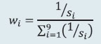
| Table 4: Risk factors constituting each component of FSSI | | Equity Market | 1. Difference between NIFTY 50 monthly returns and its maximum over a two-year rolling window
2. NIFTY 50 Market capitalisation-to-GDP ratio
3. NSE-VIX Index
4. Net Equity FPI flows | | Government Debt Market | 5. Realised volatility in 10-year G-Sec yield
6. Term Spread: Spread between 10-year G-Sec yield and 3-month T-Bill rate
7. Increase in the 10-year G-Sec yield compared to the minimum over a two-year rolling window
8. Net Debt FPI flows | | Forex Market | 9. Difference between rupee dollar exchange rate and its maximum over a two-year rolling window.
10. m-o-m appreciation/depreciation of rupee dollar exchange rate
11. GARCH (1,1) volatility of rupee dollar exchange rate
12. Difference between 3-month forward premia and its historical maximum. | | Money/Short Term Market | 13. Spread between weighted average call rate and weighted average market repo rate
14. Spread between 3-month CD rate and 3-month T-Bill rate
15. Spread between 3-month non-NBFC CP rate and 3-month T-Bill rate
16. Realised volatility of 3-month CP rate
17. Spread between 3-month OIS rate and 3-month T-Bill rate | | Corporate Bond Market | 18. Yield spread between 3-year AAA corporate bonds and 3-year G-Sec
19. Difference between 3-year BBB and 3-year AAA corporate bond yield
20. Difference between 3-year BBB corporate bond yield and its maximum | | Banking Sector | SCBs | 21. CRAR (SCBs)
22. RoA (SCBs)
23. LCR (SCBs)
24. Cost-to-Income (SCBs)
25. Stressed Assets Ratio (SCBs)
26. Banking Beta: cov(r,m)/var(m), over 2-year moving window.
r= Bank NIFTY y-o-y, m= NIFTY 50 y-o-y | | UCBs | 27. GNPA ratio (UCBs)
28. CRAR (UCBs)
29. RoA (UCBs) | | NBFC Sector | 30. GNPA ratio
31. CRAR
32. RoA
33. Spread between 3-month NBFC CP rate and 3-month T-Bill rate | | AMC-MF Sector | 34. Mutual fund redemptions: y-o-y
35. Mutual fund net inflows | | Real Sector | 36. GDP growth
37. CPI inflation
38. Current account balance as a share of GDP
39. Gross fiscal deficit as a share of GDP | |