Banking sector risks have increased since the publication of the last FSR in December 2013, as shown by the Banking Stability Indicator. Though there was a marginal improvement in asset quality, concerns remain about the liquidity and profitability aspects. Stress tests indicate higher vulnerability for public sector banks as compared to their private sector counterparts.

Various banking stability measures, based on co-movements in bank equity prices, indicate that distress dependencies within the banking system, which were rising during the second half of 2013, have remained at the same level since January 2014 mainly because of improved sentiments in stock prices. The stress tests indicate the need for a higher level of provisioning to meet the expected losses of SCBs under adverse macroeconomic conditions. However, further significant deterioration seems unlikely under normal conditions.

Scheduled Commercial Banks¹

2.1 In this section, the soundness and resilience of scheduled commercial banks (SCBs) is discussed under two broad sub-heads: banks’ performance (present status on different functional aspects and associated risks based on balance sheet data and distress dependencies based on banks’ stock prices) and their resilience (based on macro stress tests through scenarios as well as a single factor sensitivity analysis).

Performance, Vulnerabilities and Distress Dependencies

Banking Sector Risks

2.2 The risks to the banking sector as at end March 2014 increased since the publication of the previous FSR² as reflected by the Banking Stability Indicator (BSI)³, which combines the impact on certain major risk dimensions. Though there are marginal improvements in the soundness and asset quality, concerns over liquidity and profitability continue (Charts 2.1 and 2.2).

Performance

Credit and Deposit Growth

2.3 SCBs’ credit growth on a y-o-y basis declined significantly to 13.6 per cent in March 2014 from 17.1 per cent in September 2013 and 15.1 per cent in March 2013, while the decline in deposit growth from 14.4 per cent to 13.9 per cent was not as significant (Chart 2.3). SCBs’ retail portfolios, which have a share of around 19 per cent in the total loans portfolio, recorded credit growth on y-o-y basis at 16.1 per cent in March 2014, which was significantly higher than the overall credit growth.

Soundness

Capital Adequacy

2.4 The y-o-y growth in SCBs’ risk weighted assets (RWAs) declined sharply from 24.7 per cent to 12.6 per cent between September 2013 and March 2014, while the capital to risk weighted assets ratio (CRAR) improved to 12.9 per cent from 12.7 per cent (Chart 2.4).

Leverage

2.5 SCBs’ Tier I leverage ratio⁴ declined to 6.1 per cent from 6.4 per cent between September 2013 and March 2014. Among the bank groups, public sector banks recorded the lowest Tier I leverage ratio at 5.2 per cent in March 2014 (Chart 2.5).

Asset Quality

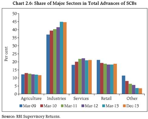
2.6 In the post-crisis period, between March 2009 and March 2013, advances to ‘industry’ recorded a compound annual growth rate (CAGR) of 24 per cent, which was significantly above the 18.1 per cent CAGR for overall advances in the same period thereby consistently and significantly raising the share of advances to the ‘industry’ sector in the total advances of SCBs to 44.7 per cent in December 2013 from 37 per cent in March 2009 (Chart 2.6).

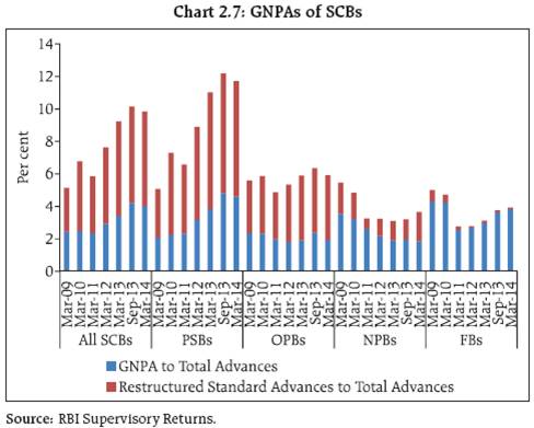
2.7 The level of gross non-performing advances (GNPAs) as percentage of total gross advances for the entire banking system declined to 4 per cent in March 2014 from 4.2 per cent in September 2013. The net non-performing advances (NNPAs) as a percentage of total net advances also declined to 2.2 per cent in March 2014 from 2.3 per cent in September 2013. This improvement in asset quality was due to the lower slippage of standard advances to non-performing advances and a seasonal pattern of higher recovery and write-offs that generally take place during the last quarter of the financial year. Sale of NPAs to asset reconstruction companies (ARCs)⁵ in the light of the Framework on Revitalising Stressed Assets could be another reason for this improvement. SCBs’ stressed advances⁶ also declined to 9.8 per cent of the total advances from 10.2 per cent between September 2013 and March 2014. Public sector banks continued to register the highest stressed advances at 11.7 per cent of the total advances, followed by old private banks at 5.9 per cent (Chart 2.7).

2.8 Though the agriculture sector accounted for the highest GNPA ratio, the share of the industry sector in restructured standard advances was high. Thus in December 2013, stressed advances in the industry sector stood at 15.6 per cent of total advances followed by the services sector at 7.9 per cent (Chart 2.8).

2.9 There are five sub-sectors: infrastructure (which includes power generation, telecommunications, roads, ports, airports, railways [other than Indian Railways] and other infrastructure), iron and steel, textiles, mining (including coal) and aviation services which contribute significantly to the level of stressed advances. The share of these five stressed sub-sectors to the total advances of SCBs is around 24 per cent, with infrastructure accounting for 14.7 per cent. Share of these five sub-sectors in total advances is the highest for public sector banks which is 27.3 per cent (Chart 2.9).

2.10 A sector-wise and size-wise analysis of the asset quality shows that the GNPA ratio of public sector banks was significantly higher than the other bank groups (Chart 2.10).

2.11 The trend of y-o-y growth in GNPAs outstripping the y-o-y growth in advances, which started from the quarter ended September 2011, continues although the gap in the growth rates is narrowing (Chart 2.11).

Profitability

2.12 Return on assets (RoA) of all SCBs remained unchanged at 0.8 per cent while return on equity (RoE) declined further from 10.2 per cent to 9.6 per cent between September 2013 and March 2014. Lower interest income and higher provisioning sharply impacted the growth in profit after tax (PAT) (Table 2.1).

2.13 The PAT growth of bank groups differs significantly. The new private banks were able to maintain a healthy growth in their PAT at 19.7 per cent during 2013-14 against a contraction of 30.7 in the PAT of public sector banks during the same period (Chart 2.12). As a result there was a sharp decline in the contribution of public sector banks to total PAT of SCBs (from 68.9 per cent to 41.5 per cent between March 2010 and March 2014) even though their share in the total assets⁷ of SCBs did not change much (Chart 2.13). On the other hand, the decline in both RoA and risk adjusted RoA⁸ (RRoA) was also more pronounced in public sector banks (Chart 2.14).

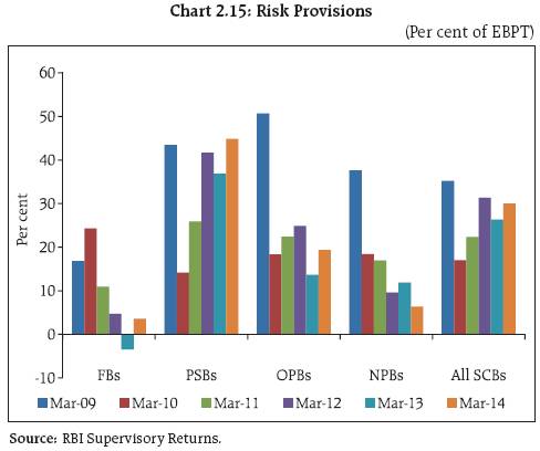
2.14 An analysis of profitability at the level of disaggregated components shows that the poorer financial performance of public sector banks as compared to the new private banks was on account of both income and provisioning. Public sector banks had lower growth in their net interest income (12.2 per cent in 2013-14) as compared to the new private banks (19.1 per cent in 2013-14) due to lower credit growth and income losses on account of higher stressed advances. Further, growth in the other operating income, which includes earnings from fee based services, forex operations and security trading of public sector banks was significantly lower at 12.2 per cent than the 18.1 per cent of new private banks during 2013-14 (Chart 2.12). On the other hand, the risk provisions of public sector banks increased to 44.8 per cent of their earnings before provisions and taxes (EBPT) in 2013-14 from 36.9 per cent in the previous financial year, whereas, these declined for new private banks to 6.4 per cent of their EBPT in 2013-14 from 11.9 per cent during the financial year ended March 2013 (Chart 2.15).

Distress Dependencies – Banking Stability Measures (BSMs)⁹

Common Distress in the System – Banking Stability Index

2.15 The Banking Stability Index (BSX), which is based on market based information, i.e., banks’ daily equity price, measures the expected number of banks that could become distressed given that at least one bank in the system becomes distressed. BSX takes into account individual bank’s probabilities of distress (PoDs)¹⁰ besides embedding banks’ distress dependency. BSX continued at the same level as observed earlier (FSR, December 2013) mainly because of improved sentiments in stock prices (Chart 2.16).

Distress Relationship among Banks

2.16 Both the Toxicity Index (TI) (which measures the average probability that a bank under distress may cause distress to another bank in the system) as well as the Vulnerability Index (VI) (which quantifies the average probability of a bank falling in distress given the occurrence of distress in the other banks in the system) showed a co-movement with BSX indicating the same level of toxicity and vulnerability of the selected banks since the publication of the previous FSR (Chart 2.17).

Resilience – Stress Tests

Macro Stress Test – Credit Risk

2.17 The resilience of the Indian banking system against macroeconomic shocks was tested through a series of macro stress tests for credit risk at system, bank group and sectoral level. These tests encompass assumed risk scenarios incorporating a baseline and two adverse macroeconomic scenarios representing medium and severe risk (Table 2.2). The adverse scenarios were derived based on up to 1 standard deviation for medium risk and 1.25 to 2 standard deviation for severe risk (10 years historical data).

System Level Credit Risk

2.18 The macro stress tests of credit risk suggest that under the baseline scenario, the GNPA ratio is expected to be around 4 per cent to 4.1 per cent during the financial year 2014-15. However, if the macroeconomic conditions deteriorate, the GNPA ratio may increase further and it could rise to around 5.1 per cent by March 2015 under a severe stress scenario. Under such a severe stress scenario, the system level CRAR of SCBs could decline to 10.6 per cent by March 2015 from 12.9 per cent in March 2014 (Chart 2.18).

Bank Group Level Credit Risk

2.19 Among the bank groups, PSBs might continue to register the highest GNPA ratio. Under a severe stress scenario, PSBs’ GNPA ratio may rise to 6.1 per cent by March 2015 from 4.6 per cent in March 2014. For NPBs it could move to 2.3 per cent from 1.9 per cent under such a severe stress scenario (Chart 2.19).

2.20 Under a severe stress scenario, PSBs may record the lowest CRAR of around 9.4 per cent by March 2015 (as against 11.4 per cent in March 2014), which is close to the minimum regulatory capital requirement of 9 per cent (Chart 2.19).

Sectoral Credit Risk

2.21 A macro stress test of sectoral credit risk revealed that among the selected seven sectors, iron & steel is expected to register the highest NPAs of around 6.7 per cent by March 2015 followed by construction and engineering in a baseline scenario. However, adverse macroeconomic shocks seem to have the maximum impact (i.e., a relatively higher rise in NPAs under a severe stress scenario) on iron & steel and engineering (Chart 2.20).

Estimation of Losses¹² for Credit Risk: Provisioning and Capital Adequacy

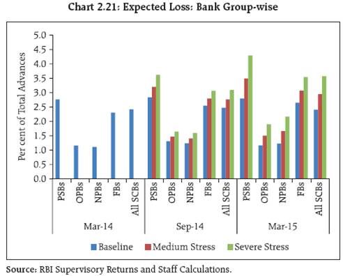
2.22 The present provisioning¹³ level of various bank groups – PSBs, OPBs, NPBs and FBs at 2.9 per cent, 1.6 per cent, 2 per cent and 3.7 per cent respectively of total advances at end March 2014, do not seem to be sufficient to meet the expected losses (EL) arising from the credit risk under adverse macroeconomic risk scenarios¹⁴. Among the bank groups, PSBs have the lowest provision coverage for EL (Chart 2.21).

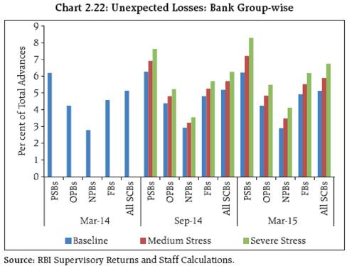
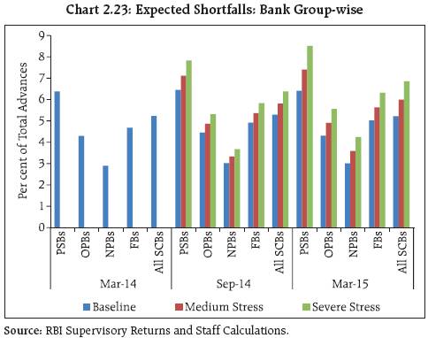
2.23 The estimated unexpected losses (UL) and expected shortfalls (ES) arising from the credit risk of various bank groups, even under severe macroeconomic stress conditions are expected to be much lower than the present level of capital (Tier I plus Tier II) maintained by them. Among the bank groups, the maximum UL is for PSBs which is 8.3 per cent of its total advances. PSBs’ ES at 8.5 cent of total advances is also the maximum. PSBs, OPBs, NPBs and FBs maintained capital at the level of 12.2 per cent, 13.7 per cent, 24.6 per cent and 35.5 per cent of total advances at end March 2014 (Charts 2.22 and 2.23).

2.24 The bank-wise¹⁵ estimation of EL and UL, arising from credit risk, shows that 17 banks were unable to meet their expected losses with their existing provisions. These banks had a 27.1 per cent share in the total advances of the select 60 banks. On the other hand, there were only three banks (with 2.2 per cent share in total advances of the select banks) which were expected to have higher unexpected losses than the total capital (Chart 2.24).

Sensitivity Analysis – Bank Level¹⁶

2.25 A number of single factor sensitivity stress tests (top-down) were carried out on SCBs (60 banks accounting for 99 per cent of the total banking sector assets) to assess their vulnerabilities and resilience under various scenarios. The resilience of commercial banks with respect to credit, interest rate and liquidity risks was studied through the top-down sensitivity analysis by imparting extreme but plausible shocks. The results are based on March 2014 data¹⁷. The same set of shocks was used on select SCBs to conduct bottom-up stress tests.

Top-Down Stress Tests

Credit Risk

2.26 The impact of different static credit shocks for banks as on March 2014 shows that the system level stressed CRAR remained above the required minimum of 9 per cent (Chart 2.25). Capital losses at the system level could be about 15 per cent in the case of a severe stress condition (shock 1). The stress test results further showed that 19 banks, sharing about 35 per cent of SCBs’ total assets, would fail to maintain required CRAR with a 100 per cent assumed rise in NPAs (shock 1). For about 9 banks, the CRAR may even go below the level of 8 per cent.

2.27 The impact of credit shocks on PSBs is more pronounced which will bring down their CRAR from 11.2 per cent to 9.1 per cent under shock (100 per cent increase in NPAs). Tier 1 CRAR will reduce from 8.4 per cent to 6.2 per cent under the assumed shock. The stressed CRAR of nationalised banks will be lower at 8.9 per cent and for SBI & associate banks it will be 9.7 per cent.

Credit Concentration Risk

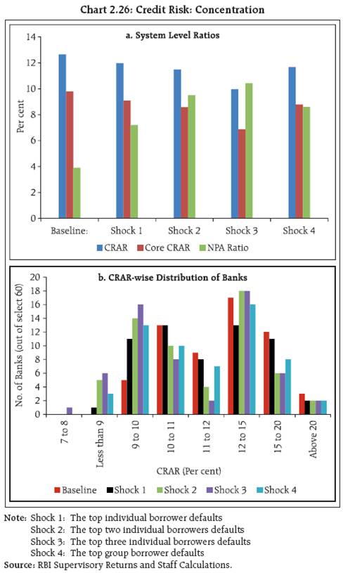
2.28 Stress tests on the credit concentration risk of banks shows that the impact under various stress scenarios was significant for about seven banks, comprising 15 per cent of assets, failing to maintain 9 per cent CRAR. Capital losses could be around 6 per cent, 10 per cent and 16 per cent at the system level under the assumed scenarios of default of the top one, two and three individual borrowers. Capital losses could be around 9 per cent at the system level under the assumed scenarios of default of top group borrowers. The impact on profit before tax (PBT) could be as high as 188 per cent with minimum of 70 per cent under the same scenarios. The direct impact on CRAR at the system level under the assumed scenarios of default of the top individual borrower, the top two individual borrowers, the top three individual borrowers and default by the top group borrowers would be 67, 117, 268 and 97 basis points. However, system level CRAR will remain above 9 per cent under these shocks (Chart 2.26).

Sectoral Credit Risk

2.29 Sectoral stress tests examined the credit risk of exposure to the broad sectors of agriculture, industry, services, retail and others. The assumed shock was an incremental increase in NPA by 5 percentage points in each sector. These tests are designed to capture the effect of a negative shock affecting important sectors. The results of a sensitivity analysis revealed that the shocks would significantly increase the system level NPAs, with the most significant effect of the single sector shock being in the industry sector (Table 2.3). The impact of the shock on capital ratios was limited given that only a portion of the credit portfolio was shocked. However, there could be a significant impact on banks’ profitability (profit before tax).

2.30 Further, using the same shocks¹⁸ at individual industry levels, the key industries which may potentially impact individual banks severely, are ranked in Table 2.4.

Interest Rate Risk

2.31 The interest rate shocks in the trading book (direct impact on the available for sale (AFS) and held for trading (HFT) portfolio of banks) under various stress scenarios resulted in a reduction in the banks’ capital adequacy ratios. The maximum impact on system CRAR was 82 basis points for an assumed shock of 250 basis point upward movement of the INR yield curve. At the bank level the stressed CRAR of six banks fell below 9 per cent. The impact of interest rate shock on the trading book for the same shock increased from the estimate of 71 basis points reported in the previous FSR. The total capital loss at the system level could be about 6.4 per cent. However, the impact in terms of profitability of banks will be significant with about 52 per cent of the banks’ profit (before tax) being lost under this shock. For the same assumed shock of 2.5 percentage points parallel upward shift of the yield curve, the impact on the held to maturity (HTM) portfolio of banks, if marked-to-market, could be about 2.8 percentage points on the capital, lower from 3.1 percentage points reported in FSR December 2013. The income impact on the banking book of SCBs could be about 24 per cent of their profit (before tax) under the shock of 2.5 percentage point parallel downward shift of the yield curve.

Solvency Stress Tests’ Results: Comparison

2.32 A single factor sensitivity analysis of the results of the solvency stress tests shows that the impact due to credit concentration on CRAR will be more severe at the system level. But the impact will be limited to a few banks having relatively high credit concentration with low capital adequacy ratios. On the other hand, the impact of the credit default in general may bring down the capital adequacy ratios below 9 per cent for more banks having comparatively high stressed advances with low capital adequacy ratios (Table 2.5).

Liquidity Risk

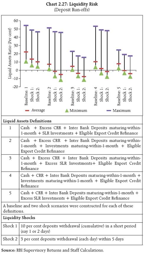
2.33 The liquidity risk analysis captures the impact of assumed deposit run-offs on banks. The analysis uses five definitions of liquid asset²⁰. As per these definitions, liquid assets comprise cash, CRR, interbank deposits and investments in different forms. Different liquid asset ratios were arrived at using various definitions under the baseline scenario. The stress scenarios were constructed to test the banks’ ability to meet a run on their deposits using only their liquid assets. It was assumed that: 1) 10 per cent of total deposits would be withdrawn in a short period (say 1 or 2 days), and 2) 3 per cent of the total deposits would be withdrawn on each day for 5 consecutive days. The analysis shows that though there was liquidity pressure under the stress scenarios, banks could withstand the assumed sudden and unexpected withdrawals by depositors with the help of their statutory liquidity ratio (SLR) investments (Chart 2.27).

2.34 Another liquidity risk analysis, based on the unutilised portion of credit lines which are sanctioned/ committed/guaranteed (taking into account the undrawn working capital sanctioned limit, undrawn committed lines of credit and letters of credit and guarantees) was attempted. The major impact was due to the utilisation of undrawn working capital limits, where 14 banks were unable to meet the credit requirements of their customers using existing liquid assets (shock1). However, the number of impacted banks was much lower at 6, if only a portion (50 per cent) of undrawn sanctioned working capital was assumed to be used by the customers (Table 2.6).

Bottom-Up Stress Tests

2.35 A series of bottom-up stress tests (sensitivity analyses) were conducted for the select sample banks²¹, with the reference date as 31 March 2014.

The results of the bottom-up stress tests carried out by select banks also testified to the banks’ general resilience to different kinds of shocks. As in the case of the top-down stress tests, the impact of the bottomup stress tests was relatively more severe on some banks with their stressed CRAR positions falling below the regulatory minimum (Chart 2.28).

2.36 The results of bottom-up stress tests for liquidity risk show a significant impact of liquidity shocks on select banks. The results also reflect that SLR investments and CRR deposits helped the banks sustain against the liquidity pressure from sudden and unexpected withdrawal of deposits by depositors to some extent (Chart 2.29).

Derivatives Portfolio of Banks

2.37 Off-balance sheet exposures in the total assets of SCBs have been recording a declining trend in the recent past. Foreign banks had a very high share of off-balance sheet assets in their total assets as compared to other bank groups (Chart 2.30).

2.38 A series of bottom-up stress tests (sensitivity analyses) on derivative portfolios were also conducted for select sample banks²², with the reference date as on 31 March 2014. The banks in the sample reported the results of four separate shocks on interest and foreign exchange rates. The shocks on interest rates ranged from 100 to 250 basis points, while 20 per cent appreciation/depreciation shocks were assumed for foreign exchange rates. The stress tests were carried out for individual shocks on a stand-alone basis.

2.39 In the sample, the mark-to-market (MTM) value of the derivatives portfolio for the banks as on 31 March 2014 varied with PSBs and PBs registering small MTM, while foreign banks had a relatively large MTM. Most of the foreign banks had negative net MTM (Chart 2.31).

2.40 The stress test results showed that the average net impact of interest rate shocks on sample banks was not high. However, the foreign exchange shock scenarios showed relatively higher impact but lower than the impact observed in September 2013 (which was due to the depreciated rupee rate prevailing at that time) (Chart 2.32).

Regional Rural Banks

Amalgamation and Scheduling of Regional Rural Banks

2.41 The second phase of amalgamation of regional rural banks (RRBs) was initiated by the Government of India in financial year 2012-13. Till the end of financial year 2013-14, 18 RRBs had been formed after amalgamating 44 RRBs. Although the pre-amalgamated RRBs were scheduled banks, the new entities formed were not scheduled. Therefore, the National Bank for Agriculture and Rural Development (NABARD) examined the issues of scheduling these RRBs and provided the Reserve Bank with suitable recommendations. Accordingly, notifications for scheduling of 16 RRBs were issued. Certificates based on inspection reports for scheduling of the remaining two RRBs are awaited from NABARD.

Scheduled Urban Co-operative Banks

Performance

2.42 At the system level²³, CRAR of scheduled urban co-operative banks (SUCBs) improved to 12.7 per cent as at end March 2014 from 12.5 per cent as at end September 2013. Though the system level CRAR of SUCBs remained above the minimum regulatory requirement of 9 per cent, at a disaggregated level eight banks failed to maintain the minimum required CRAR. The asset quality of SUCBs, measured in terms of GNPA also improved to 5.4 per cent of gross advances as at end March 2014 from 7.5 per cent as at end September 2013. There had been a significant increase in the provision coverage ratio to 71.4 per cent from 55.3 per cent during the same period (Table 2.7).

Resilience – Stress Tests

Credit Risk

2.43 A stress test for assessing credit risk was carried out for SUCBs using the data as on 31 March 2014. The impact of credit risk shocks on SUCBs’ CRAR was observed under four different scenarios²⁴. The results showed that except under the extreme scenario (100 per cent increase in GNPAs, which are classified as loss advances, where 25 out of the 51 banks failed to achieve the CRAR of 9 per cent) the system level CRAR of SUCBs remained above the minimum regulatory required level.

Liquidity Risk

2.44 A stress test on liquidity risk was carried out using two different scenarios assuming a 50 per cent and 100 per cent increase in cash outfl ows in the 1 to 28 days time bucket. It was further assumed that there was no change in cash inflows under both the scenarios. The stress test results indicate that SUCBs would be significantly impacted (27 out of 51 SUCBs under scenario I and 39 out of 51 SUCBs under scenario II) and would face liquidity stress.

Rural Co-operative Banks

Systemic Implications of Some Rural Co-operative Banks Continuing without Licenses

2.45 Pursuant to the recommendations of the Committee on Financial Sector Assessment (CFSA) the Reserve Bank had extended a one-time relaxation in licensing norms for rural co-operative banks in October 2009. Based on the relaxed licensing norms, RBI had issued licenses to eligible state co-operative banks (StCBs) and district central co-operative banks (DCCBs) on NABARD’s recommendations. As on 31 March 2014, the Reserve Bank issued banking licenses to all 32 StCBs and 348 DCCBs (out of 371 DCCBs).

2.46 The total deposits held by all the 23 unlicensed DCCBs was ` 68.3 billion at end March 2013 which had declined from ` 76.8 billion at end March 2012. NABARD conducted a snap scrutiny of these 23 unlicensed DCCBs and found that all of them were not complying with minimum capital requirements under Section 11(1) of the Banking Regulation (B.R.) Act, 1949. RBI had issued directions to these banks restraining them from accepting fresh deposits with effect from 9 May 2012 and had also issued show cause notices for placing these banks under liquidation. Many unlicensed banks are not in a position to honour depositors’ demands due to inherent financial weaknesses and liquidity problems. Keeping in view the deteriorating financial position of these unlicensed banks and based on the findings of the snap scrutiny, NABARD recommended initiating regulatory action under Section 22 of the B.R. Act, 1949. As per the directions of the Board for Financial Supervision (BFS), speaking orders rejecting the applications for carrying on the banking business were issued on 9 May 2014 to four unlicensed DCCBs and the Registrars of Cooperative Societies (RCS) were advised to appoint liquidators for these banks.

Non-Banking Financial Companies²⁵

Performance

Soundness

2.47 Every systemically important non-deposit taking NBFCs (NBFCs-ND-SI) is required to maintain a minimum capital, consisting of Tier I and Tier II capital, of not less than 15 per cent of its aggregate risk-weighted assets. The aggregate CRAR of NBFCs- ND-SI declined to 28.1 per cent in March 2014 from 28.4 per cent in September 2013 (Chart 2.33).

Asset Quality

2.48 The gross NPA ratio of NBFCs-ND-SI increased to 2.8 per cent at end March 2014 from 2.7 per cent in September 2013 (Chart 2.34).

Profitability

2.49 The RoA of NBFCs-ND-SI declined to 2.3 per cent in March 2014 from 2.5 per cent in September 2013 (Chart 2.35).

Exposure to Sensitive Sectors

2.50 Advances of NBFCs-ND-SI to the real estate sector was 4.8 per cent of the total advances and exposure to capital market (which include investments in listed instruments and advances to capital market related activities) was 8.8 per cent of total advances at end March 2014 (Chart 2.36).

Resilience – Stress Tests

System Level – Credit Risk

2.51 A stress test on credit risk for the NBFC sector (including both deposit taking and ND-SI) for the period ended March 2014 was carried out under two scenarios: (i) gross NPA increased 2 times and (ii) gross NPA increased 5 times from the current level. It was observed that in the first scenario, CRAR dropped by 1 percentage point from 28.1 per cent to 27.1 per cent, while in the second scenario it dropped by 4.1 percentage points. It may be concluded that even though there was a shortfall in provisioning under both the scenarios, CRAR of the sector was at a higher level of 24 per cent as against the minimum regulatory requirement of 15 per cent.

Individual NBFCs – Credit Risk

2.52 A stress test on credit risk for individual NBFCs for the period ended March 2014 was also carried out under two scenarios: (i) gross NPA increased 2 times and (ii) gross NPA increased 5 times from the current level. At the end of March 2014 around 8.8 per cent of the companies were unable to comply with the minimum regulatory capital requirements of 15 per cent. The non-complying percentage went up to 10.1 per cent in the case of scenario I and 11.2 per cent in scenario II.

Interconnectedness

Funding Liquidity from the Interbank Market

2.53 The interbank market is a critical source of funding for banks and had a size of around ` 8.1 trillion as of March 2014. Interbank assets as a percentage of total assets for the banking sector were around 8 per cent. The ratio however varied significantly across bank groups, with interbank business forming a major part of the portfolio for foreign banks (Table 2.8).

2.54 The PSBs as a group is the biggest net lender in the system. Nonetheless, in the short-term interbank market, they emerge as the largest borrower group. The ratio of short-term funds to total funds raised by PSBs in the interbank market was over 37 per cent (Table 2.9).

2.55 The overall dependence of new private banks and foreign banks in the interbank market was relatively higher. The ratio of funds raised from the interbank market to total outside liabilities for foreign banks and new private banks was over 34 per cent and 12 per cent respectively (Table 2.10).

2.56 The ratios given here are broad indicators of activities of different bank groups in the interbank market. There are, however, outlier banks in each group. In the case of foreign banks, the maximum interbank borrowing to outside liability ratio for a bank was around 99 per cent. This ratio for new private banks, old private banks and PSBs was around 20 per cent, 17 per cent and 15 per cent (Chart 2.37).

Trends in Connectivity and Centrality

2.57 Interconnectedness between banks as a result of activities in the interbank market, as assessed using a network analysis remained largely unchanged over the last three years. The two most significant statistics used to estimate interconnectedness: Connectivity Ratio²⁷ and Cluster Coefficient²⁸ hovered around 25 per cent and 40 per cent respectively during this period. Centrality measures were used to assess the importance of each bank in the network. The maximum eigenvalue²⁹ of the network, which is a broad indication of the stability of the system, ranged between 50 to 70 per cent. Higher maximum eigenvalue points towards increased potential contagion risks emanating from the biggest net borrower in the system (Chart 2.38).

Systemic Importance of Banks

2.58 Interbank node risk³⁰, which essentially signifies the share in interbank activities, is an indicator of the relative importance of a bank. Empirical evidence suggests that banks with high interbank node risks are also the ones with large balance sheets and which have a substantial presence in the payment and settlement system (PSS) and offbalance sheet (OBS) activities. However, the interbank node risk alone does not qualify a bank’s overall systemic importance. The bank with the highest node risk accounts for around 5 per cent of the total banking sector assets. Its share in PSS and the total OBS business is around 1 and 2 per cent. On the other hand, a few banks whose share in the total OBS business and PSS is high have a relatively lower share in the total banking sector assets and the interbank market (Chart 2.39).

Banks’ Interaction with Mutual Funds and Insurance Companies

2.59 There exists a circularity of funds between banks, mutual funds and insurance companies. These three sectors invest in each other’s assets, primarily through interbank markets. While investments by the banking sector in mutual funds and insurance companies³¹ is quite low, funds raised by the sector from the latter two is relatively higher (Tables 2.11 and 2.12).

2.60 However, when the fi gures are viewed from the perspective of mutual funds and insurance companies, they appear to be sizeable. As of March 2014, investments by mutual funds in banks as a percentage of their average assets under management (AUMs) were around 40 per cent. The figure for insurance companies stood at 13 per cent as at end March 2013 (Table 2.13).

Contagion Analysis

2.61 Based on total borrowings and the number of connections in the interbank market, each bank’s level of toxicity was estimated³³. Accordingly, a solvency contagion analysis³⁴ with network tools was used to assess distress in the banking system due to insolvency of one or more banks. The exercise is a stress test which reckons the impact of failure of a bank without taking cognisance of the probability of the failure of a bank. The failure³⁵ of the biggest net borrower in the system causes the banking system to lose around 12 per cent of its Tier I capital. However, the exercise assumes that all banks contribute to the contagion based on the degree of hit that they take on their capital. But in the Indian system PSBs carry an implicit state guarantee. Assuming that there will be no further contagion generated by the PSBs, the losses incurred by the banking system are considerably curtailed (Table 2.14).

2.62 A negative net position due to large borrowings in the interbank market may be one of the various indicators of the risk profi le of a bank. An indicator used more frequently to assess the health of a bank is the impaired asset ratio³⁶. A solvency contagion triggered by the banks with the highest impaired asset ratio reveals that not much of the banking system’s capital will be wiped out. This is due to the fact that interbank liabilities of these banks are much less. On the other hand, a liquidity contagion generated by these banks could potentially cause a far greater loss to the system (Table 2.15).

¹ Analyses of SCBs are based on their domestic operations.

² FSR – December 2013 (with reference to data at end September 2013).

³ The detailed methodology and basic indicators used under different BSI dimensions are given in Annex 2.

⁴ Tier I Leverage Ratio is defined as the ratio of Tier I capital to total assets. Total assets include the credit equivalent of off balance sheet also.

⁵ The role of ARCs has been discussed in Chapter III (Para 3.27).

⁶ For the purpose of analysing the asset quality, stressed advances are defined as GNPAs plus restructured standard advances.

⁷ Total assets include on-balance sheet assets and credit equivalent of off-balance sheet assets.

⁸ Risk adjusted RoA is defined as annual profit after tax to the risk weighted assets ratio.

⁹ The study is based on 15 major banks. These banks represent about 60 per cent of the total assets of scheduled commercial banks in India. Equity price data of the select banks have been used for the study. This model for the Indian banking system has been developed by Mr Miguel A. Segoviano, in collaboration with the Reserve Bank.

¹⁰ PoDs for banks were estimated from their equity return distributions. Under this approach, fi rst banks’ historical distributions of equity returns were estimated. Then the probability of returns falling under the historical worse 1 per cent of the cases (99 VaR) was quantified. Therefore, the PoD of a specific bank represents the probability that the bank’s equity return would fall in the tail region (historical 1 percentile).

¹¹ These stress scenarios are stringent and conservative assessments under severely adverse (hypothetical) economic conditions and should not be interpreted as forecasts or expected outcomes.

¹² The procedure adopted for estimating losses is given in Annex 2. Internationally, it is recommended to use the estimated losses (EL & UL) approach for the purpose of making provisions and capital for the next one year. For this purpose, PD is derived based on annual slippage. As the purpose of this study is to judge the adequacy of provisioning and capital levels being maintained by SCBs and not to estimate the required level of provisions and capital to be maintained for next one year, the PD used here is based on GNPAs.

¹³ Provisions include provisions for credit losses, risk provision for standard advances and provisions for restructured standard advances.

¹⁴ The stress scenarios are defined in Table 2.2 under macro stress tests (para 2.17).

¹⁵ Bank-wise estimation of EL and UL were done for the 60 SCBs which cover 99 per cent SCBs’ total assets.

¹⁶ A sensitivity analysis was done in addition to the macro stress tests; while in the former, shocks were given directly to asset quality (NPAs), in the latter the shocks were in terms of adverse macroeconomic conditions. Also, macro stress tests were done at the system, major bank group and sectoral levels, whereas the sensitivity analysis was done at aggregated system and bank levels. While the focus of macro stress tests was credit risk, the sensitivity analysis covered credit, interest rate and liquidity risks.

¹⁷ For details on the stress tests, refer to Annex 2.

¹⁸ Under the shock it is assumed that there would be an increase in NPA ratio by 5 percentage points in each sector/ industry. Accordingly the stressed NPAs are calculated. The potential losses are estimated by taking Loss Given Default (LGD) as 60 per cent on the stressed NPAs following the RBI guidelines on ‘Capital Adequacy – The IRB Approach to Calculate Capital Requirement for Credit Risk’.

¹⁹ For each bank, ranks are assigned to industries as per the estimated losses likely to be caused by the individual industry under the assumed stress scenario. The overall ranking of industries is done based on the sum of these assigned ranks.

²⁰ The guidelines on Liquidity Coverage Ratio (LCR), Liquidity Risk Monitoring Tools and LCR Disclosure Standards were issued vide circular DBOD. BP.BC 120/21.04.098/2013-14 dated 9 June 2014. LCR will be introduced in a phased manner starting with a minimum requirement of 60 per cent from 1 January 2015 and reaching minimum 100 per cent on 1 January 2019. LCR and its implementation in India is discussed in Chapter III (para 3.10).

²¹ Stress tests on various shocks were conducted on a sample of 22 select banks comprising about 70 per cent of the total assets of SCBs. The same set of shocks was used for conducting top-down and bottom-up stress tests. Details of these are given in Annex 2.

²² Stress tests on derivatives portfolios were conducted for a sample of 24 select banks (diff erent from other bottom-up stress tests) comprising about 65 per cent of total assets of SCBs. Details are given in Annex 2.

²³ System of 51 SUCBs.

²⁴ The four scenarios are: i) 50 per cent increase in GNPA (classified into sub-standard advances), ii) 50 per cent increase in GNPA (classified into loss advances), iii) 100 per cent increase in GNPA (classified into sub-standard advances), and iv) 100 per cent increase in GNPA (classified into loss advances).

²⁵ Only NBFCs-ND-SI (non-deposit taking and systemically important NBFCs) used in this analysis.

²⁶ Borrowing and lending refers to the payables and receivables on account of both fund based and non-fund based transactions in the interbank market. This includes derivative positions that banks have taken against each other. For derivatives, positive MTM and negative MTM fi gures (on a gross basis) were reckoned as receivables and payables.

²⁷ The connectivity ratio finds out how many actual connections exist in the network relative to all possible connections in it.

²⁸ Cluster coefficient is an extension of the connectivity ratio. It is based on the logic that if you have two neighbours (neighbours are banks to which direct links exist), then there is a high chance that your two neighbours are also known to each other. Suppose a bank (let us call it Bank B) has 5 neighbours (K_i), then the total possible links between these 5 banks are K_i(K_i-1), which in this case is 20. Now let us assume that in reality only 10 connections (Ei) exist between these 5 banks. Then the cluster coefficient for Bank B is E_i/K_i(K_i-1), which equals 50 per cent. The cluster coefficient for the entire network is the average of cluster coefficients of all the banks.

²⁹ Eigenvector centrality is a measure of the importance of a bank in a network. It does not just refer to the number of out-degrees or direct ‘neighbours’ that a bank has, but also depends on how connected the neighbours are. Hence, if two banks have the same number of banks that they borrow from, then the one that is likely to have a higher eigenvector centrality is the one that has a creditor bank that is also a net borrower with a larger number of other banks. Accordingly, relative scores are assigned to all nodes in the network based on the principle that connections to high-scoring nodes contribute more to the score of the node in question than equal connections to low-scoring nodes. The maximum eigenvalue refers to the score of the most dominant/most connected net borrower in the system.

³⁰ Node risk for each bank is a ratio of the total payments made plus the total received by that bank to the gross total payments made in the entire system.

³¹ The sample for the banking system includes all the scheduled commercial banks. For mutual funds and insurance companies, the sample includes 20 and 21 companies that account for over 90 per cent of the respective sector’s asset size.

³² Average AUM of Mutual Funds (Source AMFI); AUM of Insurance Companies (Source IRDA Handbook of Statistics).

³³ Eigenvector Measure of Centrality is used for the purpose.

³⁴ A solvency contagion analysis is a stress test where the gross loss to the banking system owing to a domino effect of one or more banks failing is ascertained. All the banks which have a positive net lending position vis-a-vis the failing bank will be impacted. In our analysis, this positive net position of a lender bank is deducted from its Tier I capital. If a lender bank’s Tier I capital remains above 6 per cent even after taking the hit, then the bank is considered to have survived and would not thus propagate further contagion. On the other hand, when a lender bank’s Tier I capital ratio goes below 6 per cent after the hit, then it is considered to be under distress and would propagate further contagion. We follow the round by round or sequential algorithm for simulating contagion that is now well known from Furfine (2003). Starting with a trigger bank i that fails at time 0, we denote the set of banks that go into distress at each round or iteration by D_q, q= 1,2, …n. The contagion finally ends when no more banks come under distress.

³⁵ For the purpose of this analysis, a bank is considered to be failed if its core capital adequacy ratio falls below 6 per cent. It may be noted that this is a stringent failure condition considered for the purpose of stress testing the system. The net receivables have been considered as loss for the receiving bank.

³⁶ The impaired asset ratio has been calculated as gross NPA plus restructured standard advances to gross advances.

³⁷ A liquidity contagion estimates potential loss to the system due to the failure of a net lender. The basic assumption for the analysis is that a bank will initially dip into its liquidity reserves or buffers to tide over a liquidity stress caused by the failure of a large net lender. The items considered under liquidity reserves are: (a) an excess CRR balance; (b) an excess SLR balance; (c) available marginal standing facility; and (d) available export credit refinance. If a bank is able to meet the stress with the liquidity buffers alone, then there is no further contagion. However, if the liquidity buffers alone are not sufficient, then a bank will call in all loans that are ‘callable’. For the analysis only short-term assets like money lent in the call market and other very short-term loans are assumed to be callable. Following this, a bank may survive or may be liquidated. In this case there might be instances where a bank may survive by calling in loans, but in turn might propagate a contagion causing other banks to come under duress. The second assumption used is that when a bank is liquidated, the funds lent by the bank are called in on a gross basis, whereas when a bank calls in a short-term loan without being liquidated, the loan is called in on a net basis (on the assumption that the counterparty is likely to fi rst reduce its short- term lending against the same counterparty).

³⁸ The joint liquidity solvency contagion estimates the simultaneous effects due to solvency and liquidity shocks.