Executive Summary Global growth remained resilient but below its historical average, with AI-driven investment and accommodative financial conditions somewhat offsetting tariff and geopolitical headwinds. Renewed inflation risks, driven by energy prices and volatile financial markets impart greater uncertainty to the global macroeconomic and financial outlook. Amidst heightened uncertainty and volatile capital flows, domestic financial markets fluctuated intermittently in the second half of 2025-26. System liquidity remained in surplus during H2. Money market rates evolved largely in sync with system liquidity and monetary policy actions. A combination of domestic and global cues hardened long-term government bond yields and rendered equity markets volatile. The depreciation pressures in INR accentuated at the tail end of H2, breaching its previous record lows amidst concerns over West Asia conflict. While bank credit growth continued to improve and remained supportive of real economic activity, financing from non-bank sources also increased. Transmission of the policy rate to both lending and deposit rates continued in H2 and remained robust during the current easing cycle, albeit with some frictions. In recent months, the combination of sustained credit demand and persistent gap between credit and deposit growth prompted banks to increase their term deposit rates, in addition to resource mobilisation through certificate of deposits, to bridge the funding gap. Domestic economic activity also remained resilient in the second half of 2025–26, primarily driven by private consumption, supported by both rural and urban demand, GST rate rationalisation and monetary easing. Structural reforms, favourable financial conditions and government’s thrust on infrastructure spending aided investment activity. On the supply side, services remained buoyant, and manufacturing strengthened, although agricultural activity moderated due to weather disruptions. The underlying momentum in economic activity, buoyed by further progress on trade deals with major economies, bodes well for India’s overall growth outlook. Global headwinds from geopolitical tensions, volatile commodity prices and supply-chain disruptions pose downside risks to the outlook. Specifically, intensification of the West Asia conflict could strain input supplies to various downstream sectors that may be growth inhibiting. Headline inflation in India increased from historical low levels seen in October 2025 but remained below the target thereafter. The pick-up in inflation was driven by the food group where the waning of base effects led to a turnaround from deflation. Fuel group inflation remained moderate and core inflation remained contained barring precious metals. Major methodological changes brought about by the introduction of the new series have significant implications for inflation, such as higher food group inflation and lower core. The realised cost conditions: input costs, wage costs, and margins showed no major pressures up to February 2026. Contribution of imported inflation, however, has been rising and imported input cost pressures have accentuated in March. The impact of conflict-driven spikes in global energy prices is also likely through multiple channels. Going forward, India’s macroeconomic outlook remains resilient despite elevated geopolitical tensions and lingering global trade frictions. Strong fundamentals, including sustained growth, low inflation, and fiscal consolidation, provides India the wherewithal to withstand the adverse impact of heightened global uncertainties. The surge in global crude oil prices since the West Asia conflict, exacerbated by significant supply disruptions, have tilted risks to inflation on the upside and growth on the downside, which have been communicated through asymmetric fan charts, scenario, and sensitivity analysis. In navigating through these turbulent times, monetary policy in India will continue to focus on reinforcing price stability while remaining growth supportive.
I. External Environment Global growth remains below its long‑term average amidst prolonged geopolitical tensions and trade‑related uncertainty. AI‑related investment and still‑accommodative financial conditions are supporting activity, even as bouts of heightened asset price volatility reflect shifting market sentiment. Monetary policy stances in major economies remain cautious, with central banks closely monitoring these developments. Recent energy price increases due to the West Asia conflict have heightened upside inflation risks and clouded the global growth outlook. Global growth was revised upwards by multilateral agencies prior to the onset of the West Asia conflict. However, in its March Economic Outlook, the Organisation for Economic Co-operation and Development (OECD) retained its 2026 growth projection but marginally trimmed its 2027 forecast, reflecting increased medium‑term risks from the conflict. Global growth is still projected to remain below its historical average. The outlook is highly contingent on the evolving situation in West Asia: an early resolution would likely limit the damage, whereas further escalation and a protracted conflict could have a more severe impact on the global economy. At the same time, ongoing trade and policy imbroglio is reinforcing uncertainty about the outlook. Inflation outcomes remain mixed, with some key advanced economies (AEs) remaining above target amidst renewed price pressures, fuelling expectations of a faster than anticipated pivot towards policy tightening. Global equity markets have remained largely resilient, mainly supported by AI‑related technology stocks. Concerns about stretched valuations, potential spillovers on other software industries, and escalating geopolitical tensions have, however, generated episodes of turbulence. The US dollar generally depreciated till February which eased financing conditions for emerging market economies (EMEs), but strengthened after the outbreak of the West Asia conflict on safe-haven demand. Gold repeatedly scaled new highs on safe-haven demand and central bank buying, but much of the gain reversed as the West Asia conflict intensified and the dollar strengthened. Base metal prices have increased on the back of supply disruptions and a strong demand outlook. I.1 Global Economic Conditions In 2025, global economic activity displayed resilience despite high tariffs, elevated policy uncertainty and geopolitical tensions as the overall impact of tariff measures turned out to be less severe than initially anticipated. US trade deals with major partners provided relief, but the US Supreme Court’s tariff ruling, and subsequent new tariff announcements in February, have rekindled uncertainty. In its January 2026 World Economic Outlook update, the International Monetary Fund (IMF) revised up its global growth projection for 2026 by 20 bps to 3.3 per cent, mainly reflecting stronger AI-related investment and fiscal spending. It kept its 2027 projection unchanged at 3.2 per cent. After the outbreak of the conflict, the OECD presented a more cautious picture. In its March economic outlook, it retained its growth forecast at 2.9 per cent for 2026 as the adverse effects of the West Asia conflict are expected to be offset by strong momentum in tech related investment and supportive fiscal and monetary policies. However, it marginally lowered its 2027 projection by 10 bps to 3.0 per cent. Among key AEs, US real GDP growth fluctuated over the course of 2025, reflecting the impact of tariff uncertainty, geopolitical tensions, and the partial government shutdown in the fourth quarter. The underlying economic activity, however, remained broadly resilient. After strong growth in Q3:2025, GDP growth decelerated in Q4, falling short of expectations due to weaker exports and lower government spending (Table I.1). Since October 2025, nonfarm payroll gains have slowed markedly, while the unemployment rate has remained broadly stable. In March, the composite PMI declined to its 2023 lows, as robust manufacturing activity was offset by a contraction in services. Consumer sentiment, as measured by the University of Michigan survey, improved for three consecutive months through February before easing slightly in March. It, however, remains subdued relative to historical standards as inflation and job worries remain persistent. | Table I.1: Real GDP Growth | | (Per cent) | | Country | Q1-2025 | Q2-2025 | Q3-2025 | Q4-2025 | 2025(E) | 2026(P) | 2027(P) | | Quarter-on-quarter, seasonally adjusted, annualised rate (q-o-q, saar) | | Canada | 2.1 | -0.9 | 2.4 | -0.6 | 1.6 | 1.6 | 1.9 | | Euro area | 2.4 | 0.6 | 1.2 | 0.8 | 1.4 | 1.3 | 1.4 | | Japan | 1.1 | 2.4 | -2.6 | 1.3 | 1.1 | 0.7 | 0.6 | | South Korea | -0.9 | 2.7 | 5.4 | -0.6 | 1.0 | 1.9 | 2.1 | | UK | 2.6 | 0.8 | 0.3 | 0.2 | 1.4 | 1.3 | 1.5 | | US | -0.6 | 3.8 | 4.4 | 0.7 | 2.1 | 2.4 | 2.0 | | Year-on-year | | Brazil | 3.2 | 2.4 | 1.8 | 1.8 | 2.5 | 1.6 | 2.3 | | China | 5.4 | 5.2 | 4.8 | 4.5 | 5.0 | 4.5 | 4.0 | | India | 7.0 | 6.7 | 8.4 | 7.8 | 7.3 | 6.4 | 6.4 | | Indonesia | 4.9 | 5.1 | 5.0 | 5.4 | 5.0 | 5.1 | 5.1 | | Philippines | 5.4 | 5.5 | 3.9 | 3.0 | 5.1 | 5.6 | 5.8 | | Russia | 1.4 | 1.1 | 0.6 | | 0.6 | 0.8 | 1.0 | | South Africa | 0.9 | 0.7 | 2.1 | 0.8 | 1.3 | 1.4 | 1.5 | | Thailand | 3.1 | 2.8 | 1.2 | 2.5 | 2.1 | 1.6 | 2.2 | | Memo: | | World | 2025 (E) | 2026 (P) | 2027 (P) | | Year-on-year | | Output | 3.3 | 3.3 | 3.2 | | Trade volume | 4.1 | 2.6 | 3.1 | E: Estimate. P: Projection.
Notes: 1. India’s data correspond to fiscal year (April-March); e.g., 2025 pertains to April 2025-March 2026.
2. Projections for 2026 and 2027 are taken from the IMF WEO, January 2026 update.
Sources: Official statistical agencies; Bloomberg; World Economic Outlook Update, January 2026, IMF; and RBI staff estimates. | Among other AEs, Japan’s GDP was adversely affected by US tariffs, contracting in Q3:2025 as exports declined and residential investment fell due to stricter energy-efficiency standards. In Q4, GDP grew marginally supported by a rebound in residential investment and government expenditure. Fiscal expansion by the new government is expected to support near-term growth. Expansion in the PMI eased for both services and industrial activity in March. In the euro area, GDP rose in Q3 on the back of stronger investment and government spending despite a drag from net exports. Growth weakened in Q4 as investment and government outlays slowed. In Q1:2026 so far, composite PMI in the euro area signalled expansion in February, with manufacturing rebounding amid rising new factory orders. In the UK, GDP growth remained subdued in both Q3 and Q4 due to weak services activity and a decline in construction. The November UK budget is expected to support revenues and ease concerns over rising public debt. The labour market has softened, with unemployment rising to a nearly five-year high of 5.2 per cent in December and January 2026, despite recent signs of robust business activity as indicated by PMI readings. Among major EMEs, China faced headwinds in 2025 from higher tariffs, a stagnant property market, and weak domestic consumption, yet realised its 5.0 per cent growth target. Real GDP growth moderated in Q3 and Q4 as front-loaded trade effects unravelled, and gross fixed capital formation declined. Government stimulus measures helped support consumption, even as the downturn in the property sector persisted. Notably, China’s external trade registered a record surplus in 2025, driven by diversification into new markets amid higher US tariffs. However, in March 2026, the pace of PMI expansion moderated as activity softened across both manufacturing and services. Brazil’s GDP growth remained stable at 1.8 per cent (y-o-y) in Q4 as growth in services and agriculture was offset by contraction in manufacturing. Household consumption remained weak despite a fall in the unemployment rate in Q4:2025 reflecting tighter financial conditions. The composite PMI contracted in March on falling sales across both manufacturing and services. Russia’s growth weakened in Q3 due to softer net exports amidst dampened domestic demand due to increased sanctions and high interest rates. In South Africa also, GDP growth softened in Q4 due to contractions in manufacturing and mining while the services and agriculture sectors remained resilient. After a weak Q4, however, the composite PMI remained at a neutral level in Q1:2026 (up to February), indicating stable business conditions. Growth in ASEAN1 economies was revised upwards by the Asian Development Bank (ADB) in December, raising its 2025 projection by 20 bps to 4.5 per cent from the September forecast, reflecting strong Q3 performance across key economies. Growth projections for 2026 were also revised up by 10 bps to 4.4 per cent in the wake of an improved external environment and supportive public spending. Turning to high-frequency indicators, the OECD's composite leading indicators (CLIs) showed that most economies remained above their long-term trend during Q4:2025 and Q1:2026 (up to February) (Chart I.1a). The global composite PMI stayed firmly in expansion territory in February, driven by growth in both manufacturing and services sector (Chart I.1b). However, in March manufacturing activity lost momentum as output and new orders slowed. Despite disruptions from the rising tariff-related uncertainty brought about by the Liberation Day US tariff announcements, global merchandise trade volumes expanded for nine consecutive quarters through Q4:2025. The expansion was supported by bilateral trade arrangements and front-loading of exports and imports by both emerging market and advanced economies (Chart I.2a). As per the WTO (March 2026), trade volume grew by 4.6 per cent (year-on-year) in 2025, driven by stronger trade in AI-related products that are largely exempt from tariffs and favourable macroeconomic conditions. However, the WTO projects global trade growth to decelerate sharply to 1.9 per cent in 2026 due to persistent policy uncertainty and weaker global demand. During 2025, freight rates, as reflected in the Freightos Baltic Global Index stayed below 2024 average, suggesting lower pressures on shipping cost (Chart I.2b). I.2 Commodity Prices and Inflation Since Q3:2025, commodity prices, as captured by the Bloomberg Commodity Index, have gradually moved higher with intermittent spikes led by precious metals on strong safe‑haven demand (Chart I.3a). Commodity prices have diverged largely owing to sector-specific fundamentals as precious and industrial metals witnessed a sharp increase (Box I.1). Agricultural prices remained largely unchanged on ample supplies. Global food prices rose marginally in Q1:2026 as compared to Q4:2025, driven by meat, cereals and vegetable oils (Chart I.3b). Energy prices rose in Q1:2026 relative to the previous quarter, largely driven by crude oil in the wake of supply disruptions. Brent crude ended Q4:2025 on a weaker note amid ample supply but rebounded sharply in Q1:2026 on escalating tensions in West Asia in March (Chart I.3c). Gold prices rose through Q4:2025 and the first two months of 2026, supported by safe‑haven demand on persistent trade tensions, central bank buying and a softer US dollar. However, it receded in March on the back of shifting expectations on US monetary policy, dollar appreciation, higher US yields, and profit booking. Copper rose on tighter supply and uncertainty around tariff, which increased the risk premium. Aluminium and zinc rose on supply constraint and a bearish US dollar. Base metals were further supported by an improved demand outlook from China underpinned by new government stimulus measures and the economy’s shift towards green technologies. Broader West Asia tensions added to uncertainty in global commodity markets. The metal price rally, however, faded as the US dollar strengthened in March amid rising US yields and safe-haven flows (Chart I.3d).
Consumer Price Inflation Global disinflation continued, albeit at an uneven pace across advanced and emerging economies. A subdued US dollar helped ease imported inflation pressures, particularly in emerging markets with sizeable foreign‑currency exposures. As per the latest OECD Economic Outlook, heightened uncertainty around the ongoing West Asia conflict has firmed up energy prices, which is expected to increase headline inflation in 2026 and raise medium‑term inflation expectations. Box I.1 Bubble Dynamics in Gold Prices? Gold prices rose sharply since 2024, driven by escalating geopolitical tensions, a weakening US dollar, and growing expectations of monetary policy easing across major economies following the end of the global tightening cycle. Prices underwent a sharp appreciation – increasing by more than twice within a relatively short span from around US$2,060 at end-2023 to US$5,000 per ounce by February 2026 while repeatedly scaling new highs. During this period, gold ranked among the best-performing assets globally (Chart I.1.1). While part of this increase reflects strong safe-haven demand and heightened uncertainty, the pace and persistence of the rise suggest the possibility of the build-up of bubble-like dynamics during 2025. Bubbles typically feature rapid, accelerating price surges- usually referred to as explosive behaviour – followed by sharp corrections (Phillips et al., 2011). Yet, their detection remains tricky: there is no conclusive evidence that post‑surge crashes are predictable, making it difficult to distinguish irrational exuberance from rational responses to changes in fundamentals that may be latent or unobserved (Shiller, 2000). To avoid these identification issues, statistical methods focus on the time‑series properties of prices rather than directly modelling fundamentals. In particular, they exploit hallmark explosiveness of bubbles, where the data‑generating process becomes non‑stationary with an upward drift, producing increasingly rapid price increases (Evans, 1991). This has motivated the use of methodology akin to unit‑root in which the presence of a bubble corresponds to autoregressive roots exceeding unity, signalling explosive dynamics (Phillips et al., 2015). The empirics concentrate on detecting such explosive episodes in observed price series rather than inferring bubbles solely from fundamentals.  To examine this, the Right-tailed Augmented Dickey–Fuller (RADF) methodology, implemented through rolling ADF regressions on monthly data from 1960 onwards, is used to identify episodes of explosive price behaviour. While the approach is useful in detecting periods of exuberance, it is not a conclusive test for identifying asset price bubbles. It suggests explosive behaviour even when rapid price increases are driven by shifts in fundamentals, structural breaks or volatility clustering. It also does not predict the precise timing of a potential reversal. The results show that the test statistics moved above the 95 per cent critical threshold in 2025, indicating a period of statistically significant explosive dynamics in gold prices (Chart I.1.2). A sharp correction in gold prices can trigger margin calls and liquidation of leveraged positions, forcing investors to sell other financial assets and imparting volatility across markets. It can also affect portfolio allocation and market sentiment, leading to broader repricing in equities, bonds, and currencies. Overall, the evidence suggests that gold prices entered a significant phase of price escalation in 2025, consistent with bubble-like behaviour, with the sharp and persistent price surge pointing to pronounced market exuberance and a possible increase in underlying risks. References: 1. Evans, G. W. (1991). Pitfalls in testing for explosive bubbles in asset prices. American Economic Review, 81(4), 922–930. 2. Phillips, P. C. B., Wu, Y., & Yu, J. (2011). Explosive behavior in the 1990s NASDAQ: When did exuberance escalate asset values? International Economic Review, 52(1), 201–226. 3. Phillips, P. C. B., Shi, S., & Yu, J. (2015). Testing for multiple bubbles: Historical episodes of exuberance and collapse in the S&P 500. International Economic Review, 56(4), 1043–1078. 4. Shiller, R. J. (2000). Irrational exuberance. Princeton University Press. |
Headline CPI inflation has gradually eased but remains above target in some major AEs. Inflation in the US, measured by the personal consumption expenditure (PCE) price index — the Federal Reserve’s preferred inflation metric — has been broadly stable but above target. PCE inflation has witnessed a slight uptick in recent months, reflecting higher energy prices and shelter cost amid persistent services inflation. In the UK, headline inflation has been trending lower since H2:2025, mainly due to easing services inflation amid slower wage growth, although it remains above target. In the euro area, headline inflation, which had remained close to the 2.0 per cent target in Q4:2025, dipped to 1.7 per cent in January 2026, but rose thereafter to 2.5 per cent in March, largely on account of higher energy inflation. Japan’s inflation has generally eased since the last MPR with easing food and lower electricity prices (Chart I.4a). In key emerging markets, CPI inflation has generally declined since the last MPR. In Brazil, headline CPI has been gradually converging towards target on the back of monetary tightening undertaken earlier. In South Africa, headline inflation has remained within the target band with the recent decline driven by transportation costs. In Russia, CPI inflation has been on a disinflationary path. China’s headline CPI inflation remained positive, with February posting the sharpest rise since January 2023 due to Chinese New Year related spending (Chart I.4b). Since the last MPR, inflation has edged lower in some advanced economies supported by easing of services’ inflation, while inflation in key emerging markets remain contained. However, renewed pressure on energy prices has emerged as a fresh upside risk to the inflation outlook. Overall, while inflation remains contained in many economies, the recent rise in energy prices has increased upside risks, calling for cautious adjustments of monetary policy paths. I.3 Monetary Policy Stance Since October 2025, the global easing cycle has slowed. Major central banks in AEs have largely paused, while the Bank of Japan (BoJ) and Australia have embarked on a gradual tightening cycle. A few EM central banks continued easing as inflation fell, resulting in the plateauing of policy rates. Among major AEs, the Fed reduced the policy rate by 25 basis points each in its October and December meetings as a calibrated response to the downside risks to employment. It then kept rates unchanged in Q1:2026 as inflation stayed somewhat elevated, choosing to wait and assess how earlier moves and the oil shock affect the economy before adjusting policy. In this regard, the opinions of the FOMC members have increasingly diverged in recent meetings. This reflects greater uncertainty over inflation, labour-market strength, and the timing of policy easing, with policymakers divided between guarding against persistent inflation and avoiding the costs of overtightening (Chart I.5). Since September 2025, the Bank of England has shifted from active easing to a cautious pause, cutting the Bank Rate in December but pausing thereafter as inflation trends toward target. The European Central Bank has largely completed its policy easing cycle, while maintaining a flexible and data dependent approach, with decision calibrated on a meeting-by-meeting basis. Since the last MPR, the BoJ moved from holding rates at 0.5 per cent to hiking by 25 basis points to 0.75 per cent, its highest level in three decades, as confidence grew that inflation and wages were firmer on a durable basis. The BoJ kept rates unchanged in Q1:2026, choosing to wait for clearer evidence on wage growth and underlying inflation while gauging the impact of weaker activity and the oil‑price shock from West Asia tensions before considering further tightening. Among other AEs, the Reserve Bank of Australia embarked on policy tightening with rate hikes both in February and March to counter elevated inflation amid a tighter labour market. In contrast, the Bank of Canada cut the rate by 25 bps in October 2025 to support the economy and the soft labour market. It, however, kept the policy rates unchanged in its last three meetings amidst tariff related uncertainty and elevated geopolitical tensions. Likewise, New Zealand has moved from cutting rates in Q4:2025 amid slowing growth to holding policy rate steady in 2026 so far, adopting a wait‑and‑watch stance (Chart I.6a).  Among key EMEs, Brazil’s central bank unanimously lowered the Selic rate by a quarter point in March, its first cut in almost two years as economic activity remained subdued. The Bank of Russia has gradually lowered its key rate as economic growth has moved to a more balanced pace while inflation has moved closer to target. China has held its benchmark rate at 3.0 per cent for almost a year. South Africa has moved from a target range to a point target of 3.0 per cent (±1 percentage point). With improving inflation prospects, the MPC cut the policy rate by 25 bps to 6.75 per cent in November but paused in 2026 so far due to upside risks to inflation. Thailand cut its policy rate twice to support a fragile recovery and ease debt burden. Mexico also delivered a cumulative 75 basis points rate reduction as weaker growth, and projections of inflation gradually converging toward target allowed policy normalisation (Chart I.6b). I.4 Financial Markets Notwithstanding trade tensions and geopolitical flashpoints, global risk sentiment remained buoyant in late 2025 and early 2026 as inflation eased, monetary policy stayed accommodative and AI‑related optimism persisted. In contrast, March 2026 witnessed a broad correction in equities with a shift from risk‑on sentiment as the outbreak of conflict in West Asia and renewed inflation worries prompted investors to reduce exposure to risky assets. Sovereign bond yields remained elevated amid fiscal concerns, with the recent West Asia conflict adding further upward pressure. Currency markets also reflected this shift in sentiment with the US dollar strengthening on safe-haven demand recently. Most advanced and emerging market currencies came under depreciation pressure. Global equity markets gained in Q4:2025 with gains being observed in both advanced and emerging economies (Chart I.7a). Equity markets were supported by solid earnings growth, easing inflationary pressures and expectations that systemically important central banks would continue to lower interest rates in 2026. Over the Q4 of 2025, US equities registered gains, despite the longest government shutdown. The quarterly gains helped the market to deliver a double-digit return for the third straight year. The S&P 500 Index posted a nearly 16.0 per cent return for 2025 on AI related optimism, accomodative monetary policy and some progress on trade deals, though investors remained concerned over high valuations of tech stocks. Euro area also delivered positive gains in Q4 on easing inflation and improved outlook as GDP forecast for 2025 was revised upward. Japanese equities also gained in Q4 on expectations of strong growth in generative AI and higher defence spending. The formation of the new Government in Japan was perceived as that providing greater political stability and supportive of more fiscal stimulus.  In Q1:2026, equities declined as risk sentiment deteriorated amid escalating West Asia tensions that weighed on major indices. A rising US dollar has further reinforced the risk-off tone, even as overall conditions remain supported by accommodative monetary and fiscal policies in several jurisdictions. Emerging markets have outperformed developed markets, helped by dollar weakness and country‑specific factors, despite political tensions and shifting rate expectations. More recently, both advanced and emerging markets came under selling pressure following the latest FOMC decision and minutes as investors interpreted Fed policy to be hawkish, reassessed stretched technology stock valuations, and reacted to the ongoing West Asia conflict. Japanese shares initially rose on optimism about generative‑AI demand even as domestic interest rates firmed up across the curve, reflecting higher growth and inflation along with mounting concerns over fiscal discipline. Equities, however, have since slumped as rising oil prices have clouded the economic outlook. Emerging market equity benchmarks have generally remained supported by a soft US dollar, capital inflows in specific jurisdictions, and improved sentiment around artificial intelligence (with EM Asia – particularly Korea and Taiwan – benefiting from their role in the chip and memory supply chain). China’s domestically developed AI model has kept market attention on the region’s AI potential, even as renewed trade‑policy uncertainty and rising geopolitical tensions in March sparked risk‑off sentiment, leading to decline in equities in Q1:2026. Emerging markets still trade at lower forward P/E ratios than the S&P 500, supported by benign inflation and generally accommodative monetary and fiscal policies in many economies. However, global uncertainty persists driven by tensions in West Asia, uncertain tariff landscape, and risks to future path of inflation. As crude oil prices rise, there is a growing risk that the disinflation process could pause or reverse, complicating the outlook for both inflation and monetary policy (Chart I.7b). Sovereign debt levels remain high across major advanced economies, exerting upward pressure on bond yields and intensifying the imperative for central banks to rein in inflation. In most cases, this objective has either been largely achieved or is nearing completion, although the latest energy‑price shock is again posing upside risks to inflation. In the US, yields briefly softened in October 2025 on safe‑haven demand during the shutdown. However, they soon hardened, driven by hawkish Fed communication, sticky inflation prints, and monetary policy normalisation in Japan. Sovereign bond yields across major AEs largely traded in a narrow range in Q4:2025, reflecting persistent fiscal pressures and cautious monetary policy stances. In Q1:2026, bond yields generally traded with a downward bias till February amid rotation risks following the tech sell‑off, escalating geopolitical tensions, and soft Q4:2025 GDP data of the US. Markets took comfort from clearer policy signals in Japan, easing inflation across several major economies, and episodic safe‑haven demand driven by geopolitical tensions and concerns over stretched technology valuations. In March, however, yields reversed course partially and edged higher amid renewed inflation worries following the outbreak of the conflict in West Asia, prompting investors to reassess the path of global interest rates and term premia. Japanese government bond yields rose on the back of BoJ policy normalisation, persistent inflation, and expectations of expansionary fiscal policy under the new government. In March, bond yields firmed on higher crude prices (Chart I.8a). Emerging‑market bond yields were mixed through Q4:2025 and most of Q1:2026, while lower domestic inflation and expectations of easier policy in some advanced economies supported carry in several markets, yields elsewhere rose as investors reassessed inflation risks, the likely pace of rate cuts, and the impact of the West Asia conflict on fiscal and risk premia. In March, yields picked up notably in many economies amid renewed fears of energy‑driven inflation (Chart I.8b).  Currency markets remained turbulent in 2025, especially the US dollar, which stayed subdued and highly sensitive to risk sentiment and policy expectations, though investor enthusiasm in AI and the resulting capital flows into US equities provided some support to the dollar. The US dollar fell over 9.0 per cent in 2025 against major currencies, as looming Fed rate cuts narrowed yield differentials even as worries over US fiscal deficit and political uncertainty intensified. The US dollar remained broadly unchanged in Q4:2025, with intermittent rallies driven by a hawkish Fed tone, the release of strong Q3 GDP data and safe‑haven flows. Thereafter, it has traded with a depreciating bias, reflecting weak data and deteriorating sentiment, though receiving support from safe‑haven demand during the West Asia conflict. Overall, after remaining subdued for most of Q1:2026, the dollar firmed toward the end of the quarter on renewed safe‑haven demand and still‑elevated inflation. Higher forex volatility in G7 currencies often coincided with a weaker US dollar, but this negative correlation has waned in March as safe‑haven flows and a hawkish repricing of Fed expectations have produced several recent positive readings, with volatility spikes often accompanying a stronger dollar (Chart I.9). The MSCI emerging market currency index posted gains in Q4:2025 but declined in Q1:2026, as the West Asia conflict in March triggered renewed currency pressures and portfolio outflows amid a strengthening US dollar. While AI‑related optimism and expansionary fiscal policies – provide a supportive backdrop, capital flows remain volatile amid headwinds from tariff uncertainty, geopolitical tensions, and shifting Fed policy expectations (Chart I.10 a & b). 
 I.5 Conclusion The global economy faces significant headwinds from escalating geopolitical tensions, persistent trade frictions, rising public debt, and volatility around AI‑driven equity valuations. Global growth has been resilient but remains below its historical average, while disinflation is uneven and could be reversed by the recent rise in energy prices. Overall, the outlook for 2026 points to a moderate expansion and it remains highly sensitive to shifts in the geopolitical landscape and energy‑driven inflation risks. The balancing of conflicting objectives would require cautious calibration of monetary policy paths while minimising the cost of adjustment. _________________________________________________________________________________
II. Liquidity Conditions and Financial Markets System liquidity remained in surplus during H2 supported by the Reserve Bank’s liquidity augmenting measures. Domestic financial markets exhibited bouts of volatility amidst global uncertainty. Overnight rates in the money market evolved in sync with policy rate and prevailing liquidity conditions. Transmission to lending and deposit rates continued and bank credit growth improved in H2. Sectoral trends indicate strengthening of credit growth across segments. Introduction During H2:2025-26, global financial markets generally remained resilient, before turning volatile amidst heightened geopolitical tensions due to conflict in West Asia. Domestic financial markets displayed intermittent volatility amidst global uncertainties and volatile capital flows. The Monetary Policy Committee (MPC) reduced the policy rate by 25 basis points (bps) during H2, taking the cumulative reduction to 125 bps since February 2025. Moderation in system liquidity surplus in early H2 was reversed through calibrated injections of durable liquidity. Overnight money market rates largely moved in line with the evolving liquidity conditions. Monetary policy transmission was aided by a healthy passthrough to lending and deposit rates during H2. Bank credit growth continued to improve and remained supportive of real economic activity. The financing from non-bank sources also increased. II.1 Liquidity Conditions and the Operating Procedure of Monetary Policy The Reserve Bank of India (RBI) Act, 1934 requires the Reserve Bank to place the operating procedure relating to the implementation of monetary policy and changes thereto from time to time, if any, in the public domain.1 During H2:2025-26, the MPC reduced the policy repo rate by 25 bps in the December meeting. Moreover, the MPC decided to maintain the neutral stance adopted in June 2025. The Reserve Bank also reduced the cash reserve ratio (CRR) by 100 bps to 3.0 per cent of net demand and time liabilities (NDTL) in a staggered manner during September-November 2025.2 The CRR cuts supported system liquidity during H2. Effective December 15, 2025, the definition of reporting fortnight for banks was changed along with a change in the CRR maintenance cycle. As per the new definition, a reporting cycle is defined as the period from the first day to the fifteenth day of each calendar month and the sixteenth day to the last day of each calendar month, both days inclusive. The changes in reporting cycle imply that the number of days in the first reporting cycle of the month (15 days) may be different from the second reporting cycle (which can vary from 13-16 days) with attendant implications for demand for reserves within the reserve maintenance period. Moreover, the number of reporting cycles in a year is now standardised to 24 as against 26-27 reporting fortnights in the earlier system. Drivers and Management of Liquidity System liquidity, as measured by the net balances under the liquidity adjustment facility (LAF), moderated in H2:2025–26 from a large surplus in H1 (Chart II.1). On a net basis, average daily absorption under the LAF declined to ₹1.43 lakh crore in H2, as compared with ₹2.29 lakh crore in H1. The expansion in currency in circulation (CiC) and volatile capital flows were principal drivers of liquidity conditions in H2. System liquidity remained in surplus during H2:2025- 26, except for a few intermittent occasions when tax payments withdrew liquidity from the banking system.3 System liquidity moderated in Q3, reflecting the increase in CiC during the festive season and the Reserve Bank's foreign exchange operations. It was partly offset by the reduction in the CRR and the Reserve Bank's purchase of securities through open market operations (OMOs). Liquidity conditions improved in Q4, as a sharp rise in CiC was more than offset by liquidity injection through OMO purchases, long-term USD/INR Buy/Sell swap auctions, and term repo auctions (Table II.1). 
| Table II.1: Liquidity – Key Drivers and Management | | (₹ crore) | | | 2024-25 | 2025-26 | | H1 | H2 | H1 | Q3 | Q4* | H2* | | Drivers | | | | | | | | (i) CiC [withdrawal (-) /return (+)] | 29,247 | -2,42,234 | -74,052 | -1,25,023 | -2,08,489 | -3,33,512 | | (ii) Net Forex Purchases (+)/ Sales (-) | 70,402 | -3,61,635 | -1,41,591 | -3,28,665 | 14,632 | -3,14,033 | | (iii) GoI Cash Balances [build-up (-) / drawdown (+)] | -2,04,802 | 2,98,531 | -3,44,103 | 74,298 | 26,974 | 1,01,272 | | (iv) Excess Reserves [build-up (-) / drawdown (+)] | -15,839 | 16,655 | 14,376 | 17,884 | -6,663 | 11,221 | | Management | | | | | | | | (i) Net OMO Purchases (+)/ Sales (-) | -24,040 | 2,83,386 | 2,39,223 | 1,81,435 | 4,06,900 | 5,88,335 | | (ii) Required Reserves [including both change in NDTL and CRR] | -55,613 | 76,450 | 15,674 | 1,67,530 | -17,776 | 1,49,754 | | (iii) Term Repo Auctions | - | 1,82,964 | 25,731 | - | 1,36,504 | 1,62,235 | | Memo Item | | | | | | | | (i) Long term Forex Swaps Buy/Sell (+)/ Sell/Buy (-)^ | - | 2,19,245 | - | 46,147 | 1,80,738 | 2,26,885 | | (ii) Net Absorption (+)/ Injection (-) as at end-period | 84,651 | 1,30,261 | 56,274 | 28,123 | 2,15,148 | 2,15,148 | Notes: 1. (+) / (-) sign suggests accretion to / depletion of banking system liquidity.
2. Data pertain to the last reporting day of the respective period.
3. *: Data for Q4 and H2:2025-26 are up to Mar 15, 2026.
4. ^: approximate values.
Source: RBI. | With liquidity conditions remaining in surplus, banks’ recourse to the marginal standing facility (MSF) averaged at ₹0.02 lakh crore during H2:2025-26, same as in H1, while daily balances under the standing deposit facility (SDF) increased from an average of ₹1.84 lakh crore in H1 to ₹2.20 lakh crore in H2. The Reserve Bank remained nimble and agile in its liquidity management operations to ensure sufficient liquidity in the banking system and facilitate transmission in money market (Box II.1). On a review of liquidity conditions and the outlook, the Reserve Bank undertook several measures including OMO purchases, buy/sell forex swaps and long term repos during H2 to inject durable liquidity into the banking system (Table II.2). | Table II.2: Reserve Bank’s Liquidity Measures during 2025-26 | | (₹ crore) | | Measures | H1:2025-26 | H2:2025-26 | FY:2025-26 | | CRR Cut | 62,500* | 1,87,500* | 2,50,000* | | OMO Purchase Auctions | 2,39,203 | 5,00,000 | 7,39,203 | | USD/INR Buy/Sell Swap Auctions | | 2,26,885* | 2,26,885* | | Term Repo Auctions | 25,731 | 1,36,504 | 1,62,235 | | Total | 3,27,434 | 10,50,889 | 13,78,323 | Note: * indicates approximate value.
Source: RBI. |
Box II.1: Optimal Level of Liquidity Central banks actively manage liquidity conditions in the banking system to ensure that the operating target remains aligned to the policy rate, hovering within the interest rate corridor. The guiding principle of liquidity management of the Reserve Bank, as reiterated in the revised liquidity management framework of September 2025, is to align the weighted average call rate (WACR) with the policy repo rate. Liquidity mismatches could lead to deviation of the operating target from the policy rate, hampering monetary policy transmission (Kavediya and Pattanaik, 2016). Excessive liquidity surplus over a prolonged period runs the risk of driving short term interest rates to ultra-low levels, distorting risk perceptions and engendering asset price bubbles. Moreover, persistently large surplus liquidity tends to lull market participants to a state of complacency in which they get accustomed to large liquidity. In contrast, large deficit (shortage) in the banking system liquidity raises borrowing costs for banks, which constricts lending capacity, impede monetary transmission and potentially undermine financial stability. Therefore, it becomes essential to assess the optimal level of system liquidity in consonance with the monetary policy stance. Against this backdrop, an attempt is made to estimate the adequate level of liquidity in the banking system which is consistent with the guiding principle of RBI’s liquidity management, ie., aligning the spread (weighted average call rate over policy repo rate) with the prevailing liquidity conditions (Liq) – net LAF. Considering the well-known asymmetry in transmission across surplus and deficit regimes (RBI, 2021), two separate estimations, each for the phase of surplus and deficit liquidity have been undertaken based on daily data for the period January 2012 to March 2026. Since the extent of the impact of liquidity may vary within a particular phase depending on the initial conditions, this heterogeneous impact is estimated by fitting a non-linear function. Accordingly, fractional polynomial model is fitted using the standard eight-element powers set separately for surplus and deficit liquidity conditions.4 The best-fit model for each regime is selected using Royston-Sauerbrei closed testing procedure (Royston and Sauerbrei, 2008) based on likelihood ratio tests. The fitted curves are specified below. Spread = 0.58-0.5*log (Liq+3.3); for Liq < 0 (Deficit phase) Spread = -0.03-0.07 Liq2 + 0.01 Liq3; for Liq > 0 (Surplus phase) Accordingly, the best-fit curves for the surplus and deficit liquidity period are plotted in Chart II.1.1. The relationship shows that the increase in liquidity is inversely related to the spread; moreover, the relationship is found to be non-linear. The impact of excess liquidity on the spread diminishes significantly beyond a point. The curve flattens as excess liquidity rises, suggesting that large excess liquidity does not have substantial incremental impact on the spread beyond a threshold. However, under deficit conditions, the spread becomes unbounded at higher levels of deficit. The findings suggest that surplus liquidity in the range of 0.6 to 1.1 per cent of NDTL is likely to keep the spread between 5 to 10 bps below the repo rate, while liquidity deficit in the range of 0.4 to 0.7 per cent of NDTL is likely to keep the WACR above the repo rate between 5 to 10 bps. As evident from the findings, keeping the WACR aligned to the repo rate entails different levels of liquidity in deficit and surplus conditions. Moreover, the extent of alignment is also contingent on the level of the surplus/ deficit. References: 1. Kavediya, R. and Pattanaik, S. (2016), “Operating Target Volatility: Its Implications for Monetary Policy Transmission”, Reserve Bank of India Occasional Papers Vol. 37, No. 1&2, 2016. 2. Reserve Bank of India, (2021), “Report on Currency and Finance”. 3. Royston, P. and Sauerbrei, W. (2008). Multivariable Model-Building: A Practical Approach to Regression Analysis Based on Fractional Polynomials for Modelling Continuous Variables. John Wiley & Sons, Hoboken. | The Reserve Bank conducted several variable rate repo (VRR) and variable rate reverse repo (VRRR) operations of varying maturities to modulate transient liquidity and align the rates in the overnight segment to the policy rate. Overall, 44 VRR and 7 VRRR auctions were conducted in H2:2025:26. As on March 15, 2026, reserve money (M0) expanded by 5.8 per cent (y-o-y) as against 3.7 per cent a year ago, reflecting expansion in CiC. Adjusted for the CRR change, growth in reserve money stood at 10.7 per cent (6.2 per cent a year ago). As on March 15, 2026, growth (y-o-y) in money supply (M3) rose to 10.7 per cent from 9.4 per cent a year ago with faster growth in aggregate deposits and currency with the public. Aided by CRR cuts, the money multiplier increased to 5.99 as on March 15, 2026, from 5.72 a year ago, notwithstanding an increase in the currency-deposit ratio. II.2 Domestic Financial Markets Money market rates evolved in sync with system liquidity and monetary policy actions. A combination of domestic and global factors drove long-term government bond yields higher. Equity markets and the Indian rupee displayed two-way movements amidst volatile capital flows and evolving global risk perceptions. The West Asia conflict led to accentuated downward pressure for both equity markets and the Indian rupee in March. In the credit market, bank credit grew at a healthy pace. II.2.1 Money Market During H2:2025-26, money market rates moved in tandem with the policy repo rate and evolving liquidity conditions. The weighted average call rate (WACR) – the operating target of monetary policy – largely remained below the policy repo rate until the first half of December 2025. Thereafter, during second half of December and January, the WACR traded above the policy repo rate amidst moderation in liquidity surplus (Chart II.2a). The WACR softened subsequently on the back of several liquidity augmenting measures by the Reserve Bank. The WACR hovered largely within the policy rate corridor during H2: 2025-26, with its spread over the policy repo rate widening from (-)2 bps in October 2025 to (+)4 bps in March 2026. Volatility in the WACR, as measured by the exponential weighted moving average (EWMA)5, rose in December 2025 before moderating in February and March 2026 (Chart II.2b). Overnight rates in the collateralised segment, i.e., tri-party repo and market repo, broadly moved in line with the WACR during H2 (Chart II.3).
Money market activity remained dominated by the collateralised segments (tri-party and market repo), with their share in overnight money market volume standing at 97 per cent. The share of the uncollateralised segment, i.e., the call money market, remained largely flat at around 3 per cent (Table II.3). Mutual funds (MFs) remained the major lenders in tri-party repo, despite their share tapering by 3 percentage points to 65 per cent in H2:2025-26 from H1. In the market repo segment, however, the share of lending by mutual funds increased to 48 per cent in H2 from 40 per cent in H1. The share of foreign banks’ lending in market repo remained steady at 29 per cent in H2. On the borrowing side, public sector banks (PSBs) remained the major players in the tri-party repo, with their share increasing to 32 per cent in H2 from 28 per cent in H1, while that of private sector banks declined to 24 per cent from 28 per cent. PSBs' share in market repo borrowings increased by 2 percentage points to 8 per cent over the same period. | Table II.3: Average Volume and Share in Overnight Money Market | | (₹ lakh crore) | | | 2024-25 | 2025-26 | | H1 | H2 | H1 | Q3 | Q4 | H2 | | Call/Notice | 0.10 | 0.11 | 0.16 | 0.16 | 0.15 | 0.16 | | | (2.12) | (2.18) | (2.78) | (2.72) | (2.40) | (2.56) | | Tri-party Repo | 3.30 | 3.62 | 3.69 | 3.91 | 4.35 | 4.12 | | | (68) | (70) | (66) | (66) | (70) | (68) | | Market Repo | 1.48 | 1.42 | 1.73 | 1.87 | 1.69 | 1.78 | | | (30) | (28) | (31) | (31) | (27) | (29) | | Total | 4.88 | 5.16 | 5.57 | 5.94 | 6.19 | 6.06 | | | (100) | (100) | (100) | (100) | (100) | (100) | Notes: 1. Figures in parentheses denote share of each segment in overnight money market volume. Figures may not add up to total due to rounding off.
2. Data include working saturdays.
Sources: Clearing Corporation of India Limited F-TRAC; and RBI. |
| Table II.4: Tenor wise Break up of CD Issuances | | (₹ lakh crore) | | | 2024-25 | 2025-26 | | H1 | H2 | H1 | Q3 | Q4 | H2 | | Up to 91 Days | 3.93 | 3.74 | 3.55 | 2.07 | 2.33 | 4.40 | | | (73) | (57) | (73) | (62) | (44) | (51) | | 92-180 Days | 0.20 | 0.17 | 0.47 | 0.38 | 0.23 | 0.61 | | | (4) | (3) | (10) | (11) | (4) | (7) | | 181-365 Days | 1.22 | 2.64 | 0.84 | 0.88 | 2.71 | 3.58 | | | (23) | (40) | (17) | (27) | (51) | (42) | | Total | 5.35 | 6.56 | 4.86 | 3.32 | 5.27 | 8.59 | | | (100) | (100) | (100) | (100) | (100) | (100) | Note: Figures in parentheses denote share of each maturity profile. Figure may not add up to total due to rounding off.
Sources: Clearing Corporation of India Limited F-TRAC; and RBI staff estimates. | The term segments of the money market witnessed slower transmission compared to the overnight market, mainly due to intermittent liquidity tightness and increased uncertainty. The rates on certificates of deposit (CDs) edged up especially in Q4 as banks increased issuances to bridge the widening funding gaps amidst the rollover of maturing papers and higher credit offtake. The average spread of CDs and CPs over the policy repo rate widened substantially to 116 bps and 136 bps, respectively, in H2:2025-26 from 36 bps and 60 bps, respectively, in H1. Similarly, the average spread of treasury bills (T-Bills) over the policy repo rate moved from negative to positive territory (Chart II.3). Fresh issuances of CDs increased considerably to ₹8.6 lakh crore in H2:2025-26 from ₹4.9 lakh crore in H1, reflecting widening gap between growth in deposits and credit. Tenor-wise, share of CD issuances at the shorter tenor (up to 91-day) reduced while longer tenor issuances increased in Q4 compared to Q3 as banks sought to lock in funds for longer period to meet higher credit demand (Table II.4). The issuances of CPs in the primary market declined to ₹7.9 lakh crore during H2:2025-26 from ₹8.9 lakh crore in H1, as higher rates led to a shift towards borrowings from banks (Chart II.4a). The risk premia on CPs (spread of 3-month CP rate over 91-day T-bill rate) showed an increasing trend tracking inter alia rising uncertainty in H2 (Chart II.4b).
Non-banking financial companies (NBFCs) dominated CP issuances, with an average share of 38 per cent in H2:2025-26. The share of corporates dropped to 32 per cent in H2 from 49 per cent in H1 (Chart II.5). In terms of maturity profile, the 91-180 days segment had the largest share (53 per cent) in fresh CP issuances, followed by the 31-90 days segment (Table II.5). | Table II.5: Maturity Profile of CP Issuances | | (₹ lakh crore) | | Tenor | H1: 2024-25 | H2: 2024-25 | H1: 2025-26 | H2: 2025-26 | | 7-30 days | 0.63 | 0.51 | 0.43 | 0.66 | | | (8) | (6) | (5) | (8) | | 31-90 days | 2.35 | 2.33 | 3.10 | 1.87 | | | (31) | (28) | (35) | (24) | | 91-180 days | 3.94 | 4.24 | 4.56 | 4.24 | | | (52) | (52) | (51) | (53) | | 181-365 days | 0.64 | 1.11 | 0.86 | 1.16 | | | (8) | (14) | (10) | (15) | | Total | 7.55 | 8.19 | 8.95 | 7.93 | | | (100) | (100) | (100) | (100) | | Outstanding (as at end-period) | 3.98 | 4.43 | 4.88 | 4.60 | Notes: 1. Figures in parentheses denote share of each maturity profile.
2. Figure may not add up to total due to rounding off.
Sources: Clearing Corporation of India Limited F-TRAC; and RBI. | II.2.2 Government Securities (G-sec) Market In the government securities (G-sec) market, yields generally remained under pressure during H2:2025-26 reflecting domestic as well as global factors (Chart II.6). At the beginning of H2, yields softened reflecting the MPC’s downward revision of CPI inflation forecasts for 2025–26 and Q1:2026–27 and a decline in crude oil prices. Thereafter, yields hardened in November and December, tracking rising crude oil prices, hardening US yields and increased FPI outflows.  In January, yields continued to harden before sofenting towards the month-end in response to OMO purchases undertaken by RBI. In February, yields hardened briefly due to higher-than-expected gross market borrowings announced in the Union Budget 2026-27. Subsequently, yields moved with a softening bias as RBI conducted more OMO purchases (Chart II.6). In March, yields hardened again amidst heightened geo-political tensions in West Asia triggering a rise in crude oil prices, and government's decision to cut special excise duty on diesel and petrol. At the shorter end upto one year, yields generally softened during H2:2025-26 buoyed by a policy rate cut in December 2025 and the Reserve Bank's measures for augmenting durable liquidity (Chart II.7). The average trading volume in G-secs and T-bills in H2:2025-26 was lower than H1 (Chart II.8). The weighted average yield (WAY) on traded maturities increased by 21 bps for G-secs, while it declined by 22 bps for T-bills in H2 as compared to H1. The overall dynamics of the yield curve are captured by its latent factors, viz., level, slope and curvature6. Yields have generally hardened across the term structure (Chart II.9a). This was partly attributed to (i) increased market borrowings, (ii) higher issuance of longer-tenor state government securities (SGSs), and (iii) moderation in demand for long-tenor government securities by institutional investors. The average level of yields increased by 51 bps, while the slope of the yield curve steepened by 54 bps, reflecting the hardening bias at the longer end (Chart II.9b). The curvature, on the other hand, also increased by 60 bps. In the Indian context, the level and curvature of the yield curve are found to have more information content on future macroeconomic outcomes than the slope owing to market segmentation and preferred habitat of investors, unlike in AEs (Patra et al, 2022).7 As part of active debt consolidation, the Reserve Bank conducted seven switch auctions of G-secs amounting to ₹1,45,377 crore during H2:2025-26, on behalf of the Government of India. Based on an assement of the evolving demand conditions, the supply of long papers was reduced in H2. As a result, weighted average maturity (WAM) of G-sec issuance in H2 reduced to 17.96 years from 19.65 years in H1. The WAM of the outstanding stock, however, increased from 13.60 years at end-September 2025 to 13.70 years as at end-March 2026, while the weighted average coupon (WAC) declined from 7.20 per cent to 7.17 per cent over the same period. The weighted average spread of cut-off yields on SGS over G-sec yields of comparable maturities was 57 bps in H2:2025-26 (Chart II.10) as against 38 bps in H1. The average inter-state spread of cut-off yields on SGS of 10-year tenor (fresh issuances) was 12 bps in H2 as against 5 bps in H1.
II.2.3 Corporate Bond Market Corporate bond yields increased following G-sec yields as well as due to rising risk premia during H2:2025-26 (Chart II.11a). The risk premia widened for higher and lower rated bonds. The average bond market risk premium (the spread of 3-year AAA corporate bond yields over 3-year G-sec yields) increased from 80 bps to 109 bps for Public Sector Units (PSUs), Financial Institutions (FIs) and banks; from 107 bps to 129 bps for NBFCs and from 105 bps to 112 bps for corporates in H2 (March 2026 over September 2025), amidst mixed corporate earnings in Q3 (Chart II.11b and Table II.6). 
| Table II.6: Corporate Bonds - Rates and Spreads | | | Interest Rates
(Per cent) | Spreads (bps)
(Over corresponding risk-free rate) | | Instrument | March 2025 | September 2025 | March 2026 | March 2025 | September 2025 | March 2026 | | 1 | 2 | 3 | 4 | 5 | 6 | 7 | | Corporate Bonds | | | | | | | | (i) AAA (1-yr) | 7.76 | 6.69 | 7.40 | 115 | 100 | 171 | | (ii) AAA (3-yr) | 7.62 | 7.10 | 7.36 | 98 | 105 | 112 | | (iii) AAA (5-yr) | 7.60 | 7.20 | 7.52 | 89 | 86 | 92 | | (iv) AA (3-yr) | 8.43 | 8.20 | 8.22 | 178 | 215 | 198 | | (v) BBB-minus (3-yr) | 12.09 | 11.88 | 11.92 | 544 | 583 | 567 | Note: Yields and spreads are computed as monthly averages.
Sources: Fixed Income Money Market and Derivatives Association of India (FIMMDA); and RBI staff estimates. | Primary issuances of listed corporate bonds in domestic markets declined markedly to ₹3.3 lakh crore during H2:2025-26 (up to February 2026) from ₹4.2 lakh crore during the corresponding period of the previous year due to rising cost (Chart II.12a). Overseas issuances increased to ₹24,568 crore during H2 (up to February) from ₹22,953 crore during the same period last year. Most of the resource mobilisation in the corporate bond market (98.7 per cent) was through the private placement route. Outstanding investments by foreign portfolio investors (FPIs) in corporate bonds stood at ₹1.3 lakh crore as on March 30, 2026, with moderation in utilisation of investment limits to 15.0 per cent (Chart II.12b). Trading volume in secondary market surged to ₹8.2 lakh crore during H2 (up to February 2026) from ₹7.9 lakh crore during the corresponding period of the previous year (Chart II.12c). II.2.4 Equity Market During H2:2025-26, Indian equity markets witnessed bi-directional movements. Markets gained in October-November amidst strong corporate earnings results for Q2 and policy rate cut by the US Federal Reserve. It remained range-bound in December as caution surrounding India-US trade negotiations outweighed positive global cues from policy rate cut by the US Federal Reserve and renewed optimism on AI related developments. After declining in January on fresh tariff warnings by the US and mixed corporate earnings for Q3, markets rebounded with the announcement of landmark trade deals between India and its major trading partners – the European Union and the US. Conflict in West Asia, however, led to a sharp decline in markets since end-February, which completely erased the earlier gains. Overall, broader market indices underperformed the benchmark during H2:2025-26 leading to market normalisation (Chart II.13a). Reflecting this overall performance, the price-to-earnings (PE) ratios for the broader market indices fell sharper than the benchmark in H2. The PE ratio for the benchmark BSE Sensex declined to 19.8 at end-March 2026 from 22.2 at end-September 2025. In contrast, the PE ratio for the BSE 250 SmallCap index fell sharply to 26.3 at end-March 2026 from 34.0 at end-September 2025. The PE ratio for the BSE 150 MidCap index declined to 31.1 from 34.2 during this period. The India Volatility Index, a measure of short-term expected volatility of Nifty 50, increased to 27.9 at end-March 2026 from 11.1 at end-September 2025 amidst global tariff uncertainty and persisting geo-political tensions. While all other sectors declined, metal stocks witnessed a rally led by a rise in the global prices of precious metals (Chart II.13b).  FPIs remained net sellers in the domestic equity market in H2:2025-26. Domestic institutional investors (DIIs), especially mutual funds, acted as a counterbalancing force with net buying and provided resilience to markets (Chart II.14). Resource mobilisation in primary equity markets rose to ₹2.3 lakh crore during H2 (up to February 2026), from ₹2.0 lakh crore in H1 (Chart II.15a). Average flows through systematic investment plans (SIPs) have witnessed a sustained increase in recent years supported by policy initiatives such as the ‘Chhoti SIP’ (Chart II.15b). II.2.5 Foreign Exchange Market The foreign exchange market remained volatile during H2:2025-26, driven by shifting US policies, tariff-related uncertainty, and sharp escalation in geopolitical tensions. The US dollar index witnessed a sustained decline till January, slipping to a multi-year low, weighed down by growing US growth and fiscal sustainability concerns, and uncertainty about the duration of the US Federal Reserve’s rate-cutting cycle. With the onset of West Asia conflict at end-February, the US dollar rose sharply, reflecting the rise in safe haven demand. Emerging market (EM) currencies broadly strengthened on weakening US dollar and improved global risk appetite until January 2026, but fell thereafter amidst rising global risk-off sentiments. The Indian rupee (INR) exhibited two-way movements with a depreciating bias on the back of persistent FPI outflows, elevated corporate dollar demand and rise in global risk-off sentiments in H2. The INR appreciated from early February 2026 on the announcement of interim India-US trade deal agreement, but depreciated in March as the conflict in West Asia intensified (Chart II.16a). While implied option volatility, on average, moderated in H2 vis-à-vis H1, it remained high in the face of ongoing risk-off sentiments and rising geopolitical tensions in West Asia (Chart II.16b). In order to ensure orderly conditions in the foreign exchange market, the Reserve Bank introduced a prudential measure on March 27, 2026 that limited the net open position in INR (NOP-INR) of authorised dealers in the onshore deliverable market to within US$ 100 million at the end of each business day. This was aimed at curbing excessive speculative positioning and mitigating systemic risks. 

 Overall, the INR depreciated by 6.2 per cent against the US dollar in H2 (Chart II.17). However, despite heightened volatility in global market, the INR remained among the least volatile EM currencies during this period, supported by modest current account deficit and robust foreign exchange reserves. Forward premia exhibited sharp movements during H2:2025-26, reflecting shifting interest rate differentials and evolving global sentiments (Chart II.18). The spike in short-term premia in December was driven by capital outflows, heightened global policy uncertainty, and elevated hedging demand, effectively inverting the forward premia term structure. Forward premia eased significantly from December peak as liquidity conditions eased in the wake of liquidity augmenting measures by the Reserve Bank, including USD/INR buy-sell swap auctions. In March, forward premia shot up, reflecting elevated uncertainty in West Asia. On average, the 1-month forward premia hardened to 2.76 per cent in H2 from 1.95 per cent in H1. The 12-month premia increased to 2.54 per cent from 2.12 per cent during this period. 
 In terms of the 40-currency real effective exchange rate (REER), the INR depreciated by 3.3 per cent between September 2025 and February 2026, driven by depreciation of the INR in nominal effective terms (Chart II.19a). The depreciation of INR’s 40-currency REER was broadly in line with some major economies (Chart II.19b). Financial Conditions Overall financial conditions8 remained benign during Q3. However, with the outbreak of the West Asia crisis at end-February 2026, financial conditions tightened due to broad based hardening across the entire market spectrum (Chart II.20).
II.2.6 Bank and Non-Bank Credit Bank Credit: Aggregate Trends Bank credit recorded a robust growth during H2; 2025-26, owing to monetary policy easing and strong economic activity. Growth in bank credit of scheduled commercial banks accelerated to 13.8 per cent (y-o-y) as on March 15, 2026 from 11.0 per cent a year ago. Across bank groups, credit growth of foreign banks remained the highest at 14.7 per cent (y-o-y), followed by public sector banks and private banks (Chart II.21a). As on March 15, 2026, public sector banks accounted for the largest share of incremental credit (y-o-y). However, credit growth has accelerated for private banks in recent months leading to improvement in their share in incremental credit (Chart II.21b).
The asset quality of SCBs improved further during 2025-26 (up to December 2025), with the overall gross non-performing assets (NPA) ratio declining to 2.0 per cent in December 2025 from 2.5 per cent a year ago (Chart II.22a). Asset quality improved across all major sectors (Chart II.22b). Banks’ non statutory liquidity ratio (non-SLR) investments (comprising CPs, bonds, debentures and shares of public and private corporates) grew moderately by 2.7 per cent in H2:2025-26 (up to March 15) due to decline in commercial paper holdings (Chart II.23a). Growth in adjusted non-food credit (non-food bank credit plus banks’ non-SLR investments) increased to 13.5 per cent (y-o-y) in Q4:2025-26 (up to March 15) from 10.8 per cent in Q4:2024-25 (Chart II.23b). As on February 28, 2026, excess holdings of SLR securities by SCBs moderated to 6.3 per cent of their NDTL from 7.3 per cent at end-March 2025 as banks brought down their investment portfolio to fund credit demand (Chart II.24).
Bank Credit: A Sectoral Perspective Sectoral trends9 indicate strengthening of credit growth across major segments. Industrial credit growth remained above its long-term average, thereby supporting overall credit expansion. Although personal loans growth remained below its long-term average, it has accelerated recently (Table II.7 and Chart II.25a). Personal loans and services sector continued to drive the overall credit growth (Charts II.25a and II.25b). Within the industrial sector, credit to MSMEs10 segment remained buoyant, recording a marked acceleration and contributing significantly to overall credit growth in H2:2025-26 so far11 (Chart II.26a). The flow of credit to MSMEs was supported by regulatory measures such as the enhanced limit under the Credit Guarantee Fund Trust for Micro and Small Enterprises (CGTMSE) scheme, introduction of customised credit card scheme for micro enterprises, expansion of digital and fintech lending through the co-lending framework with banks, and the updated definition of MSMEs, among others. | Table II.7: Credit Growth | | (Y-o-y, per cent) | | Sectors/Sub-sectors | Average* | Post-COVID** | Nov-23 | Mar-24 | Sep-24 | Dec-24 | Feb-25 | Mar-25 | Jun-25 | Sep-25 | Dec-25 | Jan-26 | Feb-26 | | Bank Credit | 11.1 | 14.8 | 20.7 | 20.2 | 13.0 | 11.2 | 11.1 | 11.0 | 9.5 | 10.4 | 14.5 | 14.6 | 14.5 | | Sectoral Deployment of Bank Credit | | Agriculture (13.0) | 11.4 | 14.2 | 18.1 | 20.0 | 16.4 | 12.5 | 11.4 | 10.4 | 6.8 | 9.0 | 12.1 | 11.4 | 12.3 | | Industry (22.7) | 4.6 | 8.6 | 6.9 | 9.4 | 10.0 | 7.5 | 7.5 | 8.2 | 6.3 | 7.8 | 12.8 | 12.1 | 13.5 | | Micro and Small (5.3) | 9.8 | 17.7 | 17.9 | 15.8 | 14.5 | 9.8 | 9.6 | 8.9 | 19.2 | 22.0 | 30.4 | 31.2 | 30.4 | | Medium (2.2) | 14.4 | 19.3 | 12.9 | 14.2 | 21.4 | 19.8 | 18.0 | 18.5 | 13.2 | 14.5 | 20.4 | 22.3 | 21.0 | | MSMEs (7.5) | 10.9 | 18.1 | 16.4 | 15.3 | 16.5 | 12.8 | 12.1 | 11.8 | 17.4 | 19.7 | 27.3 | 28.5 | 27.5 | | Large (15.2) | 2.8 | 5.3 | 3.7 | 7.2 | 7.5 | 5.5 | 5.6 | 6.9 | 2.0 | 3.0 | 6.9 | 5.5 | 7.8 | | Infrastructure (7.4) | 4.0 | 5.2 | 4.1 | 8.5 | 4.4 | 1.6 | 1.7 | 2.8 | 0.8 | 5.0 | 7.2 | 6.4 | 7.9 | | Services (29.6) | 14.1 | 17.2 | 24.5 | 22.3 | 12.4 | 11.5 | 11.7 | 12.0 | 8.8 | 9.8 | 15.4 | 15.5 | 16.3 | | Services excluding NBFCs (19.7) | 12.6 | 17.6 | 27.5 | 27.3 | 14.0 | 14.1 | 13.5 | 14.4 | 11.7 | 12.7 | 15.6 | 14.4 | 14.0 | | NBFCs (9.9) | 19.6 | 16.6 | 19.2 | 13.4 | 9.4 | 6.5 | 8.1 | 7.4 | 3.1 | 3.9 | 15.1 | 17.8 | 20.9 | | Personal Loans (34.7) | 17.7 | 19.1 | 30.4 | 27.8 | 13.8 | 12.0 | 11.7 | 11.7 | 11.7 | 11.8 | 14.6 | 14.9 | 15.2 | | Personal Loans with unchanged Risk Weight (23.6) | 17.3 | 19.2 | 32.2 | 31.5 | 13.9 | 12.9 | 13.5 | 13.5 | 13.9 | 14.1 | 17.1 | 17.5 | 17.6 | | Housing (Including Priority Sector Housing) (16.9) | 16.7 | 18.8 | 36.7 | 36.5 | 12.6 | 11.1 | 11.1 | 10.7 | 9.6 | 10.1 | 11.1 | 11.1 | 11.0 | | Vehicle Loans (3.7) | 18.0 | 15.2 | 20.6 | 17.6 | 13.9 | 8.8 | 9.6 | 8.6 | 9.2 | 7.3 | 16.7 | 17.1 | 17.1 | | Education (0.8) | 8.5 | 16.2 | 23.0 | 23.7 | 17.6 | 15.8 | 15.3 | 15.1 | 14.4 | 14.0 | 14.8 | 14.0 | 13.7 | | Personal Loans with increased Risk Weight (11.1) | 18.8 | 19.0 | 27.1 | 21.3 | 13.5 | 10.4 | 8.4 | 8.3 | 7.5 | 7.1 | 9.8 | 10.0 | 10.4 | | Credit Cards (1.5) | 24.2 | 21.2 | 34.2 | 25.6 | 18.0 | 15.6 | 11.2 | 10.6 | 7.2 | 3.7 | 1.0 | 1.5 | 1.7 | | Other Personal Loans (8.7) | 20.3 | 18.9 | 27.3 | 22.8 | 13.1 | 8.8 | 7.6 | 7.5 | 7.1 | 7.4 | 11.5 | 11.6 | 12.1 | Notes: 1. Provisional data.
2. *: Simple average of growth from March 2016 to February 2026.
3. **: Simple average of growth from April 2022 to February 2026
4. Figures in parentheses against each sector and sub-sectors denote share in total non-food credit as per the latest data.
Source: RBI. |
 Among the major industrial sub-sectors, credit growth of infrastructure sector strengthened in recent months, making a significant contribution to overall industrial credit expansion. Additionally, credit growth in 'basic metal and metal product', 'chemicals and chemical products' and 'all engineering' showed sustained improvement (Chart II.26b and Table II.8).
Within the services sector, 'non-banking financial companies' (NBFCs) remained the largest recipient of bank credit, with lending to them improving following the withdrawal of the additional risk weights effective April 1, 2025 (Chart II.27). Credit to services excluding NBFCs also expanded at a steady pace. Segments such as trade and commercial real estate recorded robust growth (Chart II.27 and Table II.9).
Credit growth in the personal loans segment was driven primarily by housing loans, vehicle loans and loans against gold jewellery during H2:2025-26 (Chart II.28). Both segments of personal loans, i.e., with and without change in risk weights recorded robust growth (Table II.9). The impact of increase in risk weights has gradually moderated across major sectors and subsectors. Sustained economic growth led to increased demand for bank credit. NBFCs Credit12 Credit extended by NBFCs has also strengthened since September 2025, recording sustained double-digit growth. Retail lending continued to drive overall expansion, led by housing and vehicle loans. Industrial credit exhibited steady growth, with higher lending to infrastructure, especially power sector, underscoring the important role of NBFCs in providing formal credit to niche sectors in the economy. NBFCs credit to the services sector also expanded at a healthy pace during H2:2025–26 (up to February) (Chart II.29 and Table II.10). 
| Table II.10: Sector-wise Growth in Credit by NBFCs (including HFCs) | | (Y-o-y, per cent) | | Sector | Average* | Feb-25 | Mar-25 | Jun-25 | Sep-25 | Dec-25 | Jan-26 | Feb-26 | | NBFCs Credit | 8.7 | 10.6 | 10.6 | 8.8 | 12.4 | 14.0 | 13.9 | 13.7 | | Agriculture and Allied Activities (1.3) | 13.9 | 9.0 | 6.0 | 5.1 | 5.2 | 9.4 | 10.4 | 12.6 | | Industry (38.6) | 10.9 | 9.5 | 9.7 | 10.3 | 10.2 | 9.8 | 8.9 | 8.1 | | of which | | | | | | | | | | Infrastructure (35.4) | 10.1 | 8.7 | 9.2 | 9.1 | 9.4 | 8.9 | 8.0 | 7.1 | | of which | | | | | | | | | | Power (24.9) | 12.5 | 12.3 | 12.2 | 13.3 | 11.5 | 10.1 | 9.2 | 7.8 | | Road (0.9) | 18.3 | 31.4 | 27.7 | 6.7 | 7.6 | 7.6 | 7.7 | 5.4 | | Services (12.2) | 18.8 | 13.8 | 17.4 | 14.2 | 15.8 | 19.6 | 19.4 | 18.8 | | of which | | | | | | | | | | Transport Operators (3.0) | 14.7 | 12.8 | 12.5 | 10.9 | 9.3 | 9.0 | 8.6 | 9.8 | | Trade (2.0) | 25.9 | 26.9 | 25.1 | 18.3 | 13.3 | 16.2 | 15.7 | 22.3 | | Retail Loans (42.6) | 8.7 | 13.6 | 13.1 | 11.0 | 16.6 | 18.1 | 18.7 | 19.2 | | of which | | | | | | | | | | Housing Loans (14.4)** | -5.7 | 4.2 | 4.7 | 0.4 | 9.3 | 10.7 | 10.2 | 10.0 | | Vehicle Loans (10.6) | 18.3 | 17.9 | 16.8 | 14.8 | 14.9 | 14.3 | 14.3 | 14.1 | | Loans against gold jewellery (5.3) | 27.2 | 29.0 | 32.2 | 40.6 | 50.7 | 61.2 | 68.1 | 71.9 | | Consumer Durables (1.0) | 26.1 | 25.2 | 24.0 | 18.8 | 22.2 | 23.3 | 26.4 | 28.8 | | Other Loans (5.3)*** | -10.6 | -4.8 | -8.0 | -19.5 | -4.6 | 4.2 | 4.4 | 3.5 | Notes: 1. Provisional data.
2. *: Simple average of growth from January 2023 to February 2026.
3. **:Housing loans data also include credit from Housing Finance Companies (HFCs).
4. ***:Other loans include credit from NBFCs other than agriculture, industry, services, retail loans, and non-housing loans from HFCs.
5. Data include the impact of change of nature of business of some NBFCs.
6. Figures in parenthesis represent share within total NBFCs credit.
Sources: National Housing Bank (NHB); and RBI. | II.3 Transmission to Lending and Deposit Rates Transmission of the policy rate during the current easing cycle (from February 2025) continued in H2:2025-26 with softening of both lending and deposit rates. The policy rate cut of 25 bps in December 2025 led to a cumulative rate reduction of 125 basis points (bps). The median 1-year marginal cost of funds-based lending rate (MCLR) of scheduled commercial banks (SCBs) declined by 20 bps in H2. The weighted average lending rate (WALR) on fresh rupee loans increased by 5 bps during H2 (up to February 2026), mainly reflecting compositional shift in volume towards sectors attracting relatively higher interest rates, while it declined by 26 bps for outstanding loans. On the deposit side, the weighted average domestic term deposit rate (WADTDR) on outstanding deposits declined by 20 bps in H2:2025-26 (up to February 2026), while it firmed up by 4 bps for fresh deposits (Table II.11). The combination of sustained credit demand and persistent gap between credit and deposit growth led banks to increase their term deposit rates, especially bulk deposit rates, to bridge the funding gap in recent months. In the current easing cycle (up to February 2026), the WALR for outstanding loans declined by 87 bps. For fresh rupee loans, the WALR declined by 89 bps. The interest rate effect, relatively a better measure of pricing, declined by 92 bps, reflecting robust pass-through to fresh lending rates. A lower moderation in WALR vis-à-vis the interest rate effect suggests a shift in composition-mix towards higher interest rate loans across banks and across sectors (Box II.2). The share of the external benchmark-based lending rate (EBLR) linked loans in total outstanding floating rate loans of SCBs increased from 62.9 per cent as at end-June 2025 to 65.4 per cent as at end-December 2025. Consequently, the share of MCLR linked loans declined from 33.8 per cent to 32.0 per cent over the same period. Public sector banks (PSBs) still have a significant proportion of their loans linked to the MCLR (Chart II.30a). Private banks (PVBs) extend a large part of their loans linked to EBLR (Chart II.30b). The bulk of the external benchmark-based loans use policy repo rate as the benchmark. The MCLR and other legacy rates – based on internal benchmarks and having longer reset periods – impede the pace of policy transmission. | Table II.11: Transmission to Banks’ Deposit and Lending Rates | | (Basis points) | | Period | Repo Rate | Term Deposit Rates | Lending Rates | | WADTDR Fresh Deposits | WADTDR Outstanding Deposits | EBLR | 1-Yr. MCLR (Median) | WALR Fresh Rupee Loans | WALR Outstanding Rupee Loans | | Retail Deposits | Retail and Bulk Deposits | Retail and Bulk Deposits | Overall Effect | Interest Rate Effect# | | (1) | (2) | (3) | (4) | (5) | (6) | (7) | (8) | (9) | (10) | | Tightening Cycle May 2022 to Jan 2025 | +250 | 190 | 259 | 206 | 250 | 175 | 182 | 191 | 115 | | Easing Cycle Feb 2025 to Mar 2026* | -125 | -77 | -97 | -47 | -125 | -60 | -89 | -92 | -87 | | Memo | | H2: 2025-26* | -25 | -6 | 4 | -20 | -25 | -20 | 5 | -14 | -26 | | Dec – 2025 | -25 | -4 | 8 | -5 | -25 | -5 | -43 | -12 | -15 | | Jan – 2026 | 0 | -4 | -1 | -4 | 0 | -5 | 21 | 3 | -2 | | Feb – 2026 | 0 | -3 | -1 | -2 | 0 | 5 | -5 | -1 | -4 | Notes: 1. *: Data on WALR and WADTDR are up to February 2026. #: At constant weight.
2. Data on EBLR pertain to 32 domestic banks.
WALR: Weighted average lending rate; WADTDR: weighted average domestic term deposit rate; MCLR: Marginal cost of funds-based lending rate;
EBLR: External benchmark-based lending rate.
Sources: MPD06 return; and RBI. |
Box II.2: Decomposing Monetary Policy Transmission to Lending Rates: Price and Composition Effects in WALR The weighted average lending rate (WALR), commonly used to assess monetary policy transmission, is reflective of both changes in lending rates and shifts in the composition of credit across banks and sectors. Decomposing WALR into pure pricing effect and changes arising due to credit reallocation enables a more prescient evaluation of policy rate pass-through. Huerga and Steklacova (2008) provide an index number-based framework in which changes in aggregate interest rate can be decomposed into repricing and composition effects. Building on this insight, the analysis deconstructs the WALR using index-number theory. 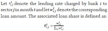 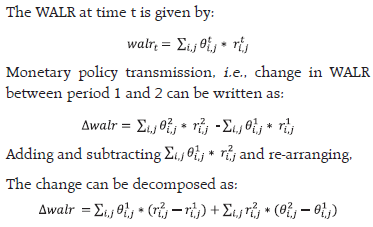 The first term represents the interest rate effect, measuring the contribution of changes in lending rates holding loan shares constant at the base period (period 1). The second term captures the composition effect, reflecting shifts in loan shares or product-mix across banks and sectors. The decomposition is implemented in levels (basis points), allowing direct interpretation of contribution to changes in aggregate WALR. Accordingly, movements in WALR may not solely reflect pricing behaviour as compositional shifts in credit allocation can amplify or dampen observed transmission. Decomposition-based diagnostics, therefore, improve the assessment of monetary policy transmission and associated lags. | Table 1: Decomposition of Weighted Average Lending Rates (February 2025-February 2026) | | | Share (per cent) | WALR (per cent) | Transmission (bps) | | Sectors | Jan-25 | Feb-26 | Jan-25 | Feb-26 | Feb-26 (Constant) | Overall | Interest Rate Effect | Weight Effect | | (1) | (2) | (3) | (4) | (5) | (6) | (7)= (5)-(4) | (8)= (6)-(4) | (9)=(7)-(8) | | Agriculture | 10.9 | 12.9 | 10.29 | 9.76 | 10.06 | -53 | -23 | -30 | | Large industry | 31.0 | 28.6 | 8.08 | 7.04 | 7.00 | -104 | -108 | 4 | | MSMEs | 9.7 | 12.7 | 9.94 | 8.76 | 8.83 | -118 | -111 | -7 | | Infrastructure | 3.6 | 3.4 | 8.55 | 7.39 | 7.59 | -116 | -96 | -20 | | Trade | 9.8 | 8.5 | 8.38 | 7.57 | 7.48 | -81 | -90 | 9 | | Professional Services | 2.6 | 2.1 | 8.75 | 8.04 | 8.05 | -71 | -70 | -1 | | Credit Cards | 0.9 | 0.7 | 37.87 | 37.15 | 37.63 | -72 | -24 | -48 | | Education | 0.2 | 0.1 | 10.76 | 9.52 | 9.68 | -124 | -108 | -16 | | Vehicle | 2.3 | 2.0 | 10.67 | 9.60 | 9.84 | -107 | -83 | -24 | | Housing | 5.6 | 4.9 | 8.70 | 7.61 | 7.63 | -109 | -107 | -2 | | Other Personal Loans | 9.4 | 11.3 | 11.27 | 10.24 | 10.38 | -103 | -89 | -14 | | Rupee Export Credit | 2.0 | 1.5 | 8.39 | 7.30 | 7.25 | -109 | -114 | 5 | | Others | 12.0 | 11.3 | 8.86 | 7.87 | 7.90 | -99 | -96 | -3 | | Aggregate | 100.0 | 100.0 | 9.33 | 8.44 | 8.41 | -89 | -92 | 3 | Notes: 1. Weight is the corresponding share of loans out of total loans.
2. Transmission during February 2025-February 2026 is calculated by subtracting the WALR of January 2025 from that of February 2026.
Sources: MPD06 return, RBI; and RBI staff calculations. | Sectoral WALRs are computed by aggregating banklevel data, which are subsequently used to arrive at the system-wide WALR. The WALR in period 1 (January 2025) was 9.33 per cent, which declined to 8.44 per cent in period 2 (February 2026). This implies that on a weighted average basis, banks have reduced their lending rates by 89 bps against a policy rate reduction of 125 bps. However, when the change in WALR is decomposed into interest rate effect and compositional shift in volume (weight effect), the pure interest rate transmission is (-) 92 bps, which is larger than a decline in overall WALR. Thus, compositional shift in lending worked in opposite direction, reducing the impact of interest rate effect by 3 bps. The above results indicate that even though lending rates declined across sectors, a shift in lending towards relatively higher interest rate sectors can partly offset this reduction through weight effect. As a result, the observed change in WALR may appear smaller, suggesting weaker policy transmission. Decomposing the change in WALR into interest rate and weight effects, therefore, provides a more realistic assessment of transmission. In essence, monetary policy transmission depends not only on change in lending rate but also on the change in composition of loan mix across sectors. Reference: Huerga, J. and Steklacova, L. (2008). An application of index numbers theory to interest rates. ECB Working Paper No. 939, September 22. | MCLR linked loans declined from 33.8 per cent to 32.0 per cent over the same period. Public sector banks (PSBs) still have a significant proportion of their loans linked to the MCLR (Chart II.30a). Private banks (PVBs) extend a large part of their loans linked to EBLR (Chart II.30b). The bulk of the external benchmark-based loans use policy repo rate as the benchmark. The MCLR and other legacy rates – based on internal benchmarks and having longer reset periods – impede the pace of policy transmission. Sectorally, PSBs have a high share of MCLR-linked loans in agriculture, large industry, infrastructure, and other personal loans (Chart II.31a). For PVBs, the shares of MCLR-linked loans are lower across sectors (Chart II.31b). The high share of MCLR-linked loans dampen the pace of transmission.
Bank group-wise, transmission to WALRs of fresh and outstanding rupee loans was higher in PVBs compared to PSBs (Chart II.32a). The large share of EBLR-based loans led to higher transmission for PVBs. However, lending rates of PVBs remained above those of PSBs (Chart II.32b). The maximum pass-through to lending rates was witnessed among foreign banks, reflecting their larger share of EBLR-linked loans.13
Sectoral analysis shows that the transmission to lending rates on fresh and outstanding loans has been broad-based. As discussed in Box II.2, the shifts in volume towards banks with relatively higher interest rates can have a bearing on overall transmission. During the current easing cycle, therefore, transmission to fresh WALR of large industry and trade has been offset by weight effect to some extent (Chart II.33). For repo-linked external benchmark loans, banks have increased their spreads (interest rate charged over and above the policy repo rate), dampening the extent of transmission (Table II.12). The spread on fresh rupee loans was the highest for education loans, followed by other personal loans, and MSME loans for domestic banks. Non-banking financial companies (NBFCs) are increasingly playing a crucial role in meeting the credit requirements of the economy. They provide last-mile credit to previously unbanked areas and offer specialised financing across sectors thereby broadening the reach of the credit channel of monetary policy transmission. However, their lending rates are generally higher than those of SCBs, mainly due to their liability structure and relatively higher risk profile of their borrowers. As a result, the extent of monetary policy transmission varies between NBFCs and SCBs (Chart II.34). | Table II.12: Spread of Weighted Average Lending Rates on Fresh Rupee Loans* | | Sectors | Jan-25 | Feb-26 | | Public sector banks | Private banks | Domestic banks | Public sector banks | Private banks | Domestic banks | | MSME Loans | 3.43 | 3.12 | 3.20 | 3.31 | 3.28 | 3.29 | | Personal Loans | | Housing | 2.09 | 2.44 | 2.34 | 2.30 | 2.51 | 2.44 | | Vehicle | 2.63 | 4.03 | 3.07 | 2.81 | 4.43 | 3.17 | | Education | 3.84 | 4.76 | 4.41 | 3.69 | 5.56 | 4.62 | | Other personal loans | 3.01 | 5.38 | 3.36 | 3.22 | 4.74 | 3.47 | Note: Other personal loans include loans other than housing, vehicle, education and credit card loans.
*: Calculated over the repo rate for loans linked to external benchmarks.
Sources: MPD06 return, RBI; and RBI staff calculations. | Transmission to deposit rates has also been robust during the current easing cycle. The weighted average domestic term deposit rates (WADTDRs) for fresh and outstanding deposits declined by 97 bps and 47 bps, respectively, during February 2025 to February 2026. Across bank groups, the transmission to both fresh and outstanding deposits was slightly higher for PSBs than PVBs; however, for fresh retail deposits it was higher for PVBs (Chart II.35a). Interest rates on fresh retail deposits moderated across tenors, although the extent varied (Chart II.35b). The share of low-cost current account and savings account (CASA) deposits declined marginally, although interest rate on savings deposit (comprising around 30 per cent of total deposits) has also declined to its lowest since its deregulation in June 2025 (Chart II.35c), helping banks to protect their net interest margins (Chart II.35d). 

| Table II.13: Interest Rates on Small Savings Instruments – Q1:2026-27 | | Small Savings Scheme | Maturity (years) | Spread$ (Percentage point) | Average G-sec yield# (Per cent) | Formula-based rate of Interest (Per cent) | GoI Announced Rate of Interest (Per cent) | Difference (Percentage point) | | (1) | (2) | (3) | (4) | (5) = (3) + (4) | (6) | (7) = (6)– (5) | | Savings Deposit | - | - | | | 4 | - | | Public Provident Fund | 15 | 0.25 | 6.83 | 7.08 | 7.1 | 2 | | Term Deposits | | | | | | | | 1 Year | 1 | 0 | 5.49 | 5.49 | 6.9 | 141 | | 2 Year | 2 | 0 | 5.70 | 5.70 | 7 | 130 | | 3 Year | 3 | 0 | 5.91 | 5.91 | 7.1 | 119 | | 5 Year | 5 | 0.25 | 6.34 | 6.59 | 7.5 | 91 | | Recurring Deposit Account | 5 | 0 | 5.91 | 5.91 | 6.7 | 79 | | Monthly Income Scheme | 5 | 0.25 | 6.31 | 6.56 | 7.4 | 84 | | Kisan Vikas Patra | 115 Months | 0 | 6.83 | 6.83 | 7.5 | 67 | | NSC VIII issue | 5 | 0.25 | 6.50 | 6.75 | 7.7 | 95 | | Senior Citizens Savings Scheme | 5 | 1.00 | 6.34 | 7.34 | 8.2 | 86 | | Sukanya Samriddhi Account Scheme | 21 | 0.75 | 6.83 | 7.58 | 8.2 | 62 | Note: Compounding frequency varies across instruments.
$: Spreads for fixing small saving rates as per the Government of India Press Release of February 2016.
#: Based on semi-annualised yield on G-sec of corresponding maturity for the period Dec 2025 - Feb 2026.
Sources: Government of India; Financial Benchmarks India Pvt. Ltd; and RBI staff calculations. | The Government of India reviewed the interest rates on various small savings instruments (SSIs) and kept them unchanged for Q1:2026-27. This led to widening gap between interest rates on SSIs and their formula-based rates (Table II.13). This gap may limit the transmission of policy rate to banks’ deposit rates, especially in an easing cycle, due to the substitution effect (Jha et al., 2025).14 The share of small savings deposit in total desopits (sum of banks' retail term deposits and small savings deposits) has increased to 19.1 per cent in January 2026 from 17.9 per cent in January 2025. It may also encourage greater migration of bank deposits to small savings thereby posing challenges for bank-based financial intermediation. II.4 Conclusion System liquidity remained in surplus during H2, except for a few sporadic instances when GST and advance tax payments withdrew liquidity from the banking system. Due to heightened global uncertainty and volatile capital flows, domestic financial markets fluctuated intermittently in H2. Money market rates evolved largely in sync with system liquidity and monetary policy actions. A combination of domestic and global factors led to hardening in long-term government bond yields. Indian equity markets demonstrated resilience, but experienced some volatility in the face of global headwinds and volatile capital flows. The Indian rupee (INR) exhibited two-way movements with depreciating bias during H2:2025-26. Following the outbreak of the West Asia conflict, both equity markets and the Indian Rupee came under accentuated pressure in March. Healthy policy transmission to bank lending rates during the current easing cycle supported robust bank credit growth. Going forward, the Reserve Bank will remain agile and nimble in liquidity management operations to ensure adequate liquidity in the banking system while safeguarding financial stability. _________________________________________________________________________________
III. Demand and Output Economic activity remained resilient in H2 of 2025–26 (up to February), primarily driven by robust domestic demand. Private consumption held up well, supported by GST rate rationalisation and monetary easing. Investment activity strengthened on the back of structural reforms, congenial financial conditions and infrastructure spending. On the supply side, services remained buoyant, and manufacturing strengthened, although agricultural activity moderated due to weather disruptions. Global headwinds from geopolitical tensions, volatile commodity prices and supply-chain disruptions pose downside risks to the outlook. Input supplies to downstream sectors need to be closely monitored for proactive policy response going forward. Recent revisions to the national accounts with an updated base year, improvements in methodology and expanded data coverage reaffirm that economic activity remained resilient in H2:2025-26, supported by robust domestic demand. Private consumption was underpinned by improving rural and urban demand conditions supported by Goods and Services Tax (GST) rate rationalisation and monetary easing. Investment activity maintained momentum, aided by ongoing structural reforms and congenial financial conditions. Government consumption also remained supportive of growth, notwithstanding continued fiscal consolidation. External demand was uneven, with resilient services exports partly offsetting softer merchandise exports in an uncertain global environment. On the supply side, services continued to be buoyant, led by high-value services, while industrial activity strengthened on the back of robust manufacturing. Agricultural activity moderated, reflecting weather-related disruptions. The Union Budget 2026-27 has proposed a six-point plan which focuses on scaling up domestic manufacturing in several strategic and frontier sectors, rejuvenating legacy industrial sectors, creating champion MSMEs, boosting infrastructure, ensuring long-term energy security and stability, and developing city economic regions. This, coupled with further progress on trade deals with major economies, bodes well for India’s overall growth outlook. Global headwinds stemming from rising geopolitical tensions, elevated commodity prices and supply-chain disruptions, however, pose downside risks to the growth outlook. III.1 Aggregate Demand Aggregate demand has maintained resilience since the October 2025 Monetary Policy Report (MPR). According to the National Statistics Office (NSO)’s Second Advance Estimates (SAE) with the new base year 2022-23, real GDP growth is placed at 7.6 per cent in 2025-26, up from 7.1 per cent in 2024-25. The pick-up was led by private final consumption expenditure (PFCE) and gross fixed capital formation (GFCF), which have expanded by 7.7 per cent and 7.1 per cent, respectively (Table III.1). PFCE contributed 4.3 percentage points to the real GDP growth, up from 3.3 percentage points a year ago. GFCF contributed 2.3 percentage points (2.1 percentage points in 2024-25), while government final consumption expenditure (GFCE) contributed 0.7 percentage points, unchanged from a year ago. In contrast, net exports acted as a drag, albeit marginally, on GDP growth (Table III.1 and Chart III.1a). | Table III.1: Real GDP Growth | | (Y-o-y growth, per cent)^ | | Item | 2024-25 | 2025-26 | Weighted Contribution* | 2024-25 | 2025-26 | | (FRE) | (SAE) | 2024-25 | 2025-26 | Q1 | Q2 | Q3 | Q4 | Q1 | Q2 | Q3 | Q4# | | Private final consumption expenditure (PFCE) | 5.8 | 7.7 | 3.3 | 4.3 | 6.1 | 5.6 | 6.0 | 5.6 | 9.2 | 8.0 | 8.7 | 5.1 | | Government final consumption expenditure (GFCE) | 6.5 | 6.6 | 0.7 | 0.7 | 7.5 | 7.0 | 7.6 | 3.6 | 5.8 | 6.6 | 4.7 | 9.4 | | Gross fixed capital formation (GFCF) | 6.4 | 7.1 | 2.1 | 2.3 | 6.5 | 6.6 | 6.3 | 6.2 | 4.9 | 8.4 | 7.8 | 7.2 | | Exports | 6.6 | 6.5 | 1.5 | 1.5 | 7.3 | 3.1 | 10.5 | 5.4 | 6.6 | 10.2 | 5.6 | 4.0 | | Imports | 5.3 | 6.4 | 1.3 | 1.5 | 8.3 | 4.6 | 2.9 | 5.5 | 7.4 | 5.9 | 8.6 | 3.6 | | GDP at market prices | 7.1 | 7.6 | 7.1 | 7.6 | 7.5 | 6.6 | 7.4 | 7.0 | 6.7 | 8.4 | 7.8 | 7.3 | Note: *: Component-wise contributions to growth do not add up to GDP growth because change in stocks, valuables and discrepancies are not included.
^: Unless specified otherwise, all discussion on growth rates in this chapter are on year-on-year (y-o-y) basis.
FRE: First revised estimates; SAE: Second advance estimates. #: implicit.
Sources: National statistics office (NSO); and RBI staff estimates. | The quarterly trajectory of GDP growth indicates that activity strengthened after a relatively softer first quarter. Real GDP growth was estimated at 6.7 per cent in Q1:2025-26, 8.4 per cent in Q2 and 7.8 per cent in Q3, with an implicit estimate of 7.3 per cent for Q4. The seasonally adjusted annualised rate (SAAR) also exhibited a similar trend, with the Q4 implicit number at 7.1 per cent (Chart III.1b). In the October 2025 MPR, real GDP growth was projected at 7.0 per cent in Q2 and 6.4 per cent in Q3, but actual growth in Q2 and Q3 turned out to be stronger at 8.4 per cent and 7.8 per cent, respectively (Chart III.2). The overshoot was mainly driven by higher-than-expected buoyancy in private consumption and a lower drag from net external demand. Overall, available high-frequency data indicate that growth remained robust in 2025-26 (up to February). Household consumption provided the main thrust, while investment demand retained traction. Net exports remained volatile.
III.1.1 Private Final Consumption Expenditure PFCE remained the mainstay of aggregate demand in 2025-26, although its share has declined under the new GDP series (base year 2022-23), reflecting both structural changes in the economy and the use of new data sources (Box III.1). As per the SAE, PFCE recorded a growth of 7.7 per cent in 2025-26, up from 5.8 per cent in 2024-25. The quarterly trajectory of PFCE growth, however, points to some moderation, with 9.2 per cent in Q1, 8.0 per cent in Q2, 8.7 per cent in Q3 and an implicit 5.1 per cent in Q4 (Table III.1). Urban demand indicators generally presented an improving picture in H2:2025-26 (Table III.2). Passenger vehicle sales registered strong double-digit growth in Q3:2025-26, before moderating in January and February 2026. Consumer durables output remained in expansionary territory in the first two months of Q4:2025-26. Domestic air passenger traffic remained volatile, but stayed in expansionary territory, on average, in Q3 and Q4. The pace of unsecured household credit accelerated – personal loans recorded robust growth in Q3 and January-February 2026, even as growth in credit card outstanding remained muted during this period. Box III.1: New Series of National Accounts - Improvements in Methodology and Coverage India’s revised national accounts series with base year 2022–23 strengthens the measurement framework through methodological improvements, enhanced data coverage and improved reconciliation between the production and expenditure sides. Methodologically, the revised series, inter alia, adopts double deflation1 in manufacturing and agriculture, uses more granular deflators, updates compilation ratios using recent survey evidence, improves the allocation of corporate-sector value added across activities using MGT-7/7A annual return filings2, and aligns quarterly estimates more closely with annual national accounts. Regarding data, it makes greater use of surveys and administrative sources, including GST, Annual Survey of Unincorporated Sector Enterprises (ASUSE), Periodic Labour Force Survey (PLFS), Household Consumption Expenditure Survey (HCES), Public Financial Management System (PFMS) and e-Vahan, while also improving the coverage of paid household services and digital/platform activities. Moreover, the incorporation of the Supply and Use Table (SUT) framework through product balancing strengthens reconciliation between production- and expenditure-side estimates that helps in reducing statistical discrepancies. The major methodological improvements, data coverage enhancements, and system integration measures are summarised in Table III.1.1. The base year revision, together with methodological improvements, has addressed several issues in India’s national accounts highlighted in the IMF’s Article IV Reports on India. One important implication is a modest shift in the measured sectoral composition of real GVA over 2022–23 to 2024–25, with a higher share for agriculture and allied activities, and lower shares for industry and services (Chart III.1.1). The increase in the agriculture share likely reflects improved measurement of crop and allied activities, updated input-output structures, and better use of season-wise source data for crops, livestock and fisheries, with some quarterly estimates apportioned from season-wise information. By contrast, the moderation in the services share is consistent with better capture of informal service activity in the revised series, including through ASUSE-based information. In absolute terms, the discrepancy as a share of GDP averaged about 2.0 per cent under the earlier series, as against around 0.3 per cent under the revised series over 2022–23 to 2025–26, pointing to improved reconciliation between the production and expenditure sides of the accounts. The revised series also yields a somewhat smoother Incremental Capital Output Ratio (ICOR) profile in recent years, suggesting lower cyclicality rather than any material change in its average level (Chart III.1.2). | Table III.1.1: Key Methodological Improvements, Data Coverage Enhancements and System Integration Measures | | Changes | Implications | | Methodological improvements | Deflation strategy | Double deflation and single extrapolation are used in manufacturing and agriculture; single deflation discontinued. | Improves separation of price and volume effects and strengthens measurement of real value added. | | Granular deflators | Wider use of CPI, WPI and unit value indices at item-group level rather than aggregate deflators. | Enhances accuracy of constant-price estimates and comparability across sectors. | | Updated rates and ratios | Compilation parameters revised using recent surveys and sectoral studies. | Improves representativeness of sectoral estimates. | | Multi-activity corporate reporting | Use of MGT-7/7A filings to allocate value added across activities rather than assigning it solely to principal activity. | Improves industry classification and sectoral GVA allocation. | | PFCE compilation | Mixed methodology, combining HCES, administrative data and commodity-flow methods; adoption of COICOP 2018 classification. | Strengthens the level and composition of private consumption and improves international comparability. | | Quarterly-annual alignment | Quarterly compilation framework aligned more closely with annual national accounts in classification and deflation practices. | Improves consistency between quarterly and annual GDP estimates and reduces revisions arising from methodological differences. | | Data and coverage enhancements | Household enterprise measurement | ASUSE provides direct benchmarks for output and value added of informal enterprises. | Improves measurement of household/ unincorporated sector production. | | Labour input information | PLFS provides employment and labour-force information used in estimating labour-intensive activities. | Strengthens estimation of household-based services and informal sector activity. | | Administrative data integration | Greater use of GST, PFMS and e-Vahan databases in compilation. | Improves timeliness and cross-validation of production and expenditure estimates. | | Coverage of household services | Explicit inclusion of hired domestic workers in GDP estimates. | Expands coverage of paid household services within GVA. | | Digital and platform economy | Improved capture of digital, platform and gig-economy activities, including informal and self-employed segments. | Enhances measurement of emerging services and digitally mediated activities. | | Integration and institutional accounts | SUT integration | Systematic integration of the SUT framework through product-balancing to reconcile supply and use. | Improves reconciliation between production and expenditure estimates and reduces statistical discrepancies. | | Government sector estimation | Enhanced use of budget documents and administrative accounts; improved treatment of NPS/OPS pensions, HRA imputation, local bodies coverage, and subsidy deflation. | Improves completeness and valuation of government output and expenditure. | | State accounts (GSDP) alignment | Revised guidelines and methodological support to states to align GSDP compilation with national accounts. | Strengthens consistency between national and state accounts and reduces reliance on allocation methods. | | Note: PFCE: Private Final Consumption Expenditure; GVA: Gross Value Added; GSDP: Gross State Domestic Product; NPS: National Pension System; OPS: Old Pension Scheme; HRA: House Rent Allowance; e-Vahan: national vehicle registration database. |
")
 Looking ahead, India’s statistical system is expected to evolve further in line with emerging international statistical standards. With the global transition from the System of National Accounts (SNA) 2008 to the forthcoming SNA 2025 framework over the next decade, further refinements, particularly in measuring the digital economy, global production arrangements and multinational enterprise activity, and in deepening the use of administrative data are expected to strengthen the robustness and transparency of national accounts. References: Ministry of Statistics and Programme Implementation (MoSPI). (2026). Press Release: Redefining Growth—India’s Revised GDP Estimates and the New Measurement Framework. Government of India. Ministry of Statistics and Programme Implementation (MoSPI). Report of the Committee on Constant Price Estimates. Government of India. Government of India. Public Financial Management System (PFMS). Ministry of Finance. | Rural demand conditions improved further. Tractor and motorcycle sales posted strong expansion in Q3 and the first two months of Q4:2025-26. Consumer non-durables output turned positive in Q3 after remaining in contraction during the first half of the year. Demand for work under the Mahatma Gandhi National Rural Employment Guarantee Act (MGNREGA) remained in contraction in Q3 and subsequent months, indicating improved employment in the rural sector. Fast-moving consumer goods (FMCG) volume growth in rural area outpaced that in urban area in Q3, while the position reversed in January-February 2026, with urban demand outpacing rural demand. | Table III.2: Indicators of Consumption | | (Y-o-y growth, per cent) | | Indicator | 2024-25 | 2025-26 | | | Q1 | Q2 | Q3 | Q4 | Q1 | Q2 | Q3 | Jan | Feb | | Urban demand | | Domestic air passenger traffic | 5.6 | 7.3 | 11.4 | 12.0 | 5.3 | -1.9 | 1.7 | 3.1 | -0.1 | | Passenger vehicle sales (wholesale) | 20.2 | -1.3 | 5.1 | 3.6 | -1.4 | -1.5 | 20.6 | 8.0# | 7.3# | | Consumer durables | 10.7 | 6.6 | 9.0 | 5.9 | 2.6 | 6.9 | 7.3 | 7.2 | 7.3 | | Personal loan | 25.6 | 13.4 | 12.0 | 11.7 | 11.7 | 11.7 | 14.4 | 14.9 | 15.2 | | Vehicle loan | 12.0 | 10.6 | 8.8 | 8.6 | 9.2 | 7.3 | 16.5 | 17.1 | 17.1 | | Credit card outstanding | 23.3 | 18.0 | 15.6 | 10.6 | 7.2 | 3.7 | 1.0 | 1.5 | 1.7 | | Rural demand | | Tractor sales | 0.5 | 0.7 | 13.5 | 17.3 | 9.2 | 30.7 | 23.2 | 43.0 | 34.2 | | Motorcycle sales | 16.8 | 10.2 | -1.9 | -3.5 | -9.2 | 5.0 | 12.0 | 20.3 | 30.8 | | Consumer non-durables | -0.2 | -2.2 | -1.6 | -2.0 | -1.5 | -2.0 | 4.1 | -2.3 | -0.6 | | Fertiliser sales | 2.4 | -7.3 | 0.4 | -9.6 | -14.7 | 30.6 | 7.5^ | | | | MGNREGA work demand | -16.1 | -16.5 | 1.7 | 6.5 | 1.3 | -21.3 | -31.8 | -25.7 | -14.2 | | FMCG sales | | Rural | | 5.7 | 9.1 | 9.5 | 8.4 | 7.7 | 2.9 | -0.5 | -0.2 | | Urban | | 1.9 | 4.0 | 3.5 | 4.1 | 4.0 | 2.3 | 2.4 | 2.4 | | All India | | 3.5 | 6.2 | 6.1 | 6.0 | 5.5 | 2.6 | 1.1 | 1.3 | Notes: #: Does not include Tata Motors. ^Fertiliser sales in Q3:2025-26 correspond to October and November 2025.
Sources: Directorate General of Civil Aviation (DGCA), Society of Indian Automobile Manufacturers (SIAM); Tractor and Mechanization Association (TMA); NSO; RBI; Ministry of Chemicals and Fertilizers (MoC&F); Ministry of Rural Development (MoRD); NielsenIQ’s Retail Audit Service; and RBI staff estimates. | According to the March 2026 round of the Reserve Bank’s urban consumer confidence survey, both the Current Situation Index (CSI) and the Future Expectations Index (FEI) moderated from the previous round. However, both current perceptions and one year ahead expectations on consumer spending have improved marginally in March 2026 compared to January 2026 (Table III.3). Labour market conditions presented a mixed picture in H2:2025-26 (Chart III.3). The worker population ratio (WPR) improved in Q4 (up to February 2026), while the labour force participation rate (LFPR) remained broadly stable with some month-to-month variation. The unemployment rate, after edging up in January 2026, moderated in February. The composition of employment shifted further towards self-employment in Q3, alongside some moderation in the share of regular salaried employment. | Table III.3: Summary of Urban Consumer Confidence based on Net Responses | | (Percentage responses) | | Main variable | Current Perceptions | One year ahead Expectations | | Jan-26 | Mar-26 | Jan-26 | Mar-26 | | Economic Situation | -3.5 | -8.6 | 29.3 | 23.1 | | Employment | -6.3 | -9.1 | 33.0 | 25.2 | | Price Level | -81.2 | -85.2 | -75.2 | -76.7 | | Income | 3.3 | 3.0 | 50.1 | 48.4 | | Spending | 78.0 | 78.4 | 80.0 | 81.2 | | Consumer Confidence Index | 98.1 | 95.7 | 123.4 | 120.2 | Note: ‘Net response’ is the difference between the percentage of respondents reporting optimism and those reporting pessimism. It ranges between -100 and 100. Any value greater than zero indicates expansion/ optimism and values less than zero indicate contraction/ pessimism. Consumer Confidence Index = 100 + Average of Net Responses on the economic situation, income, spending, employment and the price level.
Source: Urban Consumer Confidence Survey, RBI. |
III.1.2 Gross Fixed Capital Formation Gross fixed capital formation (GFCF) maintained momentum in 2025-26. As per the SAE, GFCF posted a growth of 7.1 per cent in 2025-26, up from 6.4 per cent in 2024-25. It remained the second largest contributor to the real GDP growth (Table III.1). After a softer first quarter, investment activity strengthened in the subsequent quarters, with GFCF growth at 8.4 per cent in Q2, and 7.8 per cent in Q3. High-frequency indicators pointed to sustained investment activity. Imports of capital goods recorded double digit growth in Q3:2025-26 and maintained a healthy pace during January-February 2026 (Table III.4). The production of capital goods also recorded strong growth in Q3, with a notable pick-up in February 2026. Construction-related indicators continued to display a healthy picture – cement production increased at double digit rate in Q3:2025-26 and January 2026, while finished steel consumption grew at a modest pace in Q3 although it gained momentum in February 2026. The resilience in investment activity is also borne out of survey and corporate indicators. Capacity utilisation in manufacturing improved in Q3:2025-26, and remained above both its 12-quarter moving average (QMA) and its long-period average. The interest coverage ratio (ICR) of listed private manufacturing companies improved to 9.0 in Q3:2025-26. Among service sector companies, the ICR of non-IT services firms improved, while that of IT services moderated, albeit remaining at an elevated level. Improving ICR points to strengthening the financial health of the corporate sector, which, along with benign financial conditions, should support the ongoing investment cycle (Chart III.4). | Table III.4: Indicators of Investment Demand | | (Y-o-y growth, per cent) | | Indicators | 2024-25 | 2025-26 | | Q1 | Q2 | Q3 | Q4 | Q1 | Q2 | Q3 | Jan | Feb | | Import of capital goods | 10.0 | 11.7 | 6.0 | 7.9 | 14.3 | 8.5 | 11.4 | 7.1 | 19.7 | | IIP: capital goods | 3.0 | 4.9 | 7.4 | 7.0 | 9.8 | 5.6 | 6.8 | 4.1 | 12.5 | | Finished steel consumption | 15.3 | 12.1 | 8.1 | 11.2 | 7.9 | 8.8 | 4.6 | 4.9 | 12.8 | | Cement production | 0.4 | 3.2 | 8.7 | 12.4 | 8.0 | 7.3 | 11.2 | 11.3 | 9.3 | | Sources: Directorate General of Commercial Intelligence and Statistics. (DGCI&S); NSO; Joint Plant Committee; and Office of the Economic Adviser. | On the aggregate financing side, the savings-investment gap narrowed modestly in 2024-25, with the gap between gross capital formation (GCF) and gross domestic savings (GDS) easing to 0.6 per cent of GDP from 0.8 per cent a year ago. The gross domestic investment rate – measured by the ratio of GCF to GDP at current prices – rose to 35.5 per cent in 2024-25 from 33.6 per cent in the preceding year, indicating buoyancy in capital formation. GDS also increased to 34.9 per cent of GDP in 2024-25 from 32.8 per cent a year ago, reflecting lower dissaving by the general government sector alongside an increase in household net financial saving (Chart III.5a).3 These dynamics suggest a reduced dependence on external savings for domestic investment. The sectoral saving-investment balances also indicate an easing in financing pressures during 2024-25. The household sector remained the net supplier of funds, imparting stability to financing conditions. The resource gap of private non-financial corporations narrowed, while fiscal consolidation reduced general government dissaving (Chart III.5b). Overall, the narrowing of the aggregate resource gap suggests an improvement in the financing conditions that drive the investment cycle. III.1.3 Government Consumption As per the SAE, GFCE increased by 6.6 per cent in 2025-26, marginally higher as compared to 6.5 per cent in the previous year. GFCE recorded a growth of 4.7 per cent in Q3:2025-26 and an implicit growth of 9.4 per cent in Q4. The Central Government’s revenue expenditure, net of interest payments and major subsidies, contracted during Q2 and Q3, partly on account of a decline in grants-in-aid to State governments/UTs. It is, however, expected to register high growth in Q4 to achieve its full year revised estimates (Chart III.6). As per the Union Budget 2026-27, revenue expenditure net of interest payments and major subsidies for 2026-27 is budgeted to grow by 6.7 per cent, higher than 3.1 per cent in the revised estimates for 2025-26. 
 The Central Government’s gross fiscal deficit (GFD)4 stood at 4.4 per cent of GDP in 2025-26(RE), adhering to its medium-term target of a GFD below 4.5 per cent by 2025-26 (as announced in the Union Budget 2021-22). This was achieved through rationalisation of expenditure, and higher than budgeted non-tax revenue receipts. For 2026-27, the Central Government budgeted a lower GFD at 4.3 per cent of GDP, thus adhering to the path of fiscal prudence. Further consolidation is budgeted mainly through containment of revenue expenditure to 10.5 per cent of GDP [from 10.8 per cent in 2025-26 (RE)], while maintaining capital expenditure at 3.1 per cent of GDP. Revenue expenditure to capital outlay ratio5 (RECO) has remained low at 4.4, suggesting the preservation of expenditure quality (Table III.5).  During 2025-26 (April-February), the Central government’s capital expenditure grew by 14.5 per cent, while revenue expenditure excluding interest payments and major subsidies contracted by 6.0 per cent (y-o-y). On the receipts side, the gross tax revenue posted a growth of 6.7 per cent, driven by corporation tax, union excise duties, and customs duties. Within direct taxes, corporation tax recorded a robust growth of 12.4 per cent (y-o-y), compared to 1.9 per cent during the corresponding period of last year. Income tax collections grew at 0.9 per cent during 2025-26 (April-February), substantially lower than 22.0 per cent during the previous year. Under indirect taxes, growth of GST collections moderated to 5.1 per cent from 11.6 per cent a year ago, while growth in customs and union excise duty collections accelerated. Monthly GST collections6 (Centre plus States) averaged at ₹1.94 lakh crore during 2025-26 (Chart III.7). The consolidated GFD of State governments and Union Territories is budgeted at 3.3 per cent of GDP for 2025–26, the same as the provisional estimates of 2024-25 (Table III.6). States have projected an increase of 23.0 per cent in revenue receipts, driven by both tax and non-tax revenues. State governments' continued emphasis on capital expenditure led to an improvement in their RECO ratio and a rise in capital outlay to GDP ratio in 2025-26 (BE) [Chart III.8]. Going forward, the Centre’s enhanced allocation of ₹2 lakh crore towards ‘Special Assistance to States for Capital Investment’ announced in the Union Budget 2026-27 would provide further boost to States’ capex. | Table III.5: Central Government Finances | | (Per cent of GDP) | | Indicator | 2023-24 | 2024-25 | 2025-26 (RE) | 2026-27 (BE) | | 1. Revenue receipts | 9.1 | 9.2 | 9.4 | 9.0 | | a. Tax revenue (Net) | 7.7 | 7.6 | 7.5 | 7.3 | | b. Non-tax revenue | 1.3 | 1.6 | 1.9 | 1.7 | | 2. Non-debt capital receipts | 0.2 | 0.1 | 0.2 | 0.3 | | 3. Revenue expenditure | 11.6 | 10.9 | 10.8 | 10.5 | | a. Interest payments | 3.5 | 3.4 | 3.6 | 3.6 | | b. Major subsidies | 1.4 | 1.2 | 1.2 | 1.0 | | 4. Revenue expenditure excluding interest payments and major subsidies | 6.7 | 6.4 | 6.1 | 5.9 | | 5. Capital expenditure | 3.2 | 3.2 | 3.1 | 3.1 | | 6. Capital outlay | 2.6 | 2.6 | 2.5 | 2.4 | | 7. Total expenditure | 14.8 | 14.1 | 13.9 | 13.6 | | 8. Gross fiscal deficit | 5.5 | 4.8 | 4.4 | 4.3 | | 9. Revenue deficit | 2.5 | 1.7 | 1.5 | 1.5 | | 10. Primary deficit | 2.0 | 1.4 | 0.8 | 0.7 | | Memo: | | Ratio of Revenue Expenditure to Capital Outlay | 4.4 | 4.2 | 4.4 | 4.4 | Notes: RE: Revised Estimates; and BE: Budget Estimates.
Sources: Union Budget Documents and RBI staff estimates. | The deficit indicators of States during 2025-26 (April-January), as a proportion of BE, were higher than the comparable period of the previous year (Chart III.9a), primarily due to a moderation in revenue receipts. States’ goods and services tax (SGST), the major source of tax revenue, recorded decelerated growth, partly reflecting rationalisation of GST rates. State excise collections, stamp duties and registration fees, on the other hand, registered robust growth. States’ revenue expenditure grew at a slower pace than a year ago, while capital expenditure recorded a turnaround (Chart III.9b). In 2025-26, the Centre’s gross market borrowings through issuance of dated securities amounted to ₹14.61 lakh crore, marginally lower than the budgeted estimates of ₹14.82 lakh crore. In pursuit of active debt consolidation, the Reserve Bank conducted 14 switch auctions/ operations on behalf of the Central Government (amounting to ₹2.75 lakh crore) involving the substitution of shorter-maturity securities with those of longer-maturity. The weighted average yield on issuances during 2025-26 declined to 6.7 per cent from 7.0 per cent in 2024-25. The weighted average maturity of borrowings also declined to 18.9 years from 20.7 years in the previous year. State Governments/UTs raised gross market borrowings of ₹12.76 lakh crore in 2025-26, higher than ₹10.73 lakh crore in the previous year (Table III.7). The Centre’s gross market borrowings and net borrowings for 2026-27 are budgeted at ₹17.20 lakh crore and ₹11.73 lakh crore, respectively. The WMA limit for Central Government for H1 of 2026-27 has been fixed at ₹2.5 lakh crore to meet the temporary mismatches between receipts and payments. Consequent on the Reserve Bank entering into an agreement with the Government of National Capital Territory of Delhi (GNCTD) on January 05, 2026, the revised aggregate WMA limit for State Governments/ UTs, including GNCTD has been fixed at ₹61,008 crore as against the existing limit of ₹60,118 crore. 
| Table III.6: State Government Finances - Key Fiscal Indicators | | (Per cent of GDP) | | Item | 2023-24 (A) | 2024-25 (PA) | 2025-26 (BE) | | Revenue deficit | 0.3 | 0.6 | 0.2 | | Gross fiscal deficit | 2.9 | 3.3 | 3.3 | | Primary deficit | 1.2 | 1.7 | 1.5 | Note: Data pertain to 31 States/UTs.
A: Actuals; PA: Provisional Accounts; BE: Budget Estimates.
Sources: Budget Documents of States/UTs and Comptroller and Auditor General (CAG) of India. |
III.1.4 External Demand Global demand conditions weakened amid elevated trade tensions and policy uncertainty in H2:2025-26.7 The outbreak of West Asia conflict since end-February further dented global demand. Despite the challenging global environment, merchandise exports held ground, increasing marginally by 0.8 per cent in H2 (October-February). Continued resilience in services exports supported India's external demand. With merchandise imports growing at a higher pace than exports, the trade deficit expanded to US$ 155.7 billion in H2:2025-26 (October-February) from US$ 115.9 billion in H2:2024-25 (October-February) [Chart III.10]. Export performance varied across sectors. The growth in merchandise exports during September-February 2025-26 was primarily led by electronic goods, engineering goods, meat, dairy and poultry products, drugs and pharmaceuticals, and marine products. The impact of higher US tariffs was evident in lower shipments to the US, particularly from the impacted sectors, viz., gems and jewellery, automobiles and certain automobile parts, textiles and readymade garments, although diversification to other markets partly offset the impact. Major sectors that dragged down overall exports included petroleum products, rice, gems and jewellery, textiles, and plastic and linoleum (Chart III.11). | Table III.7: Government Market Borrowings | | (₹ crore) | | | 2024-25 | 2025-26 | | | Centre | States | Total | Centre | States | Total | | Net borrowings | 11,62,879 | 7,53,345 | 19,16,224 | 11,32,834 | 9,03,887 | 20,36,721 | | Gross borrowings | 14,00,697 | 10,73,310 | 24,74,007 | 14,61,000 | 12,76,430 | 27,37,430 | | Sources: Government of India (GoI); and RBI staff estimates. |
The growth in merchandise imports during September-February 2025-26 was driven by higher imports of gold, electronic goods, silver, fertilisers, and machinery, electrical and non-electrical. In contrast, petroleum, crude and products, iron and steel, pulses, coal, coke and briquettes, and chemical material and products contributed negatively (Chart III.12). Gold imports at US$ 52 billion grew sharply by 78.5 per cent (y-o-y) during this period reflecting a steep rise in prices, while petroleum, crude and products contracted by 5.6 per cent. Services exports expanded by a healthy 8.9 per cent during 2025-26 (April-February), although it moderated from 13.1 per cent in the same period of last year. Driven by software and business services on sustained global demand, India remained one of the top five service-exporting countries worldwide in terms of export growth in 2025-26 (April-January). In H2:2025-26 (October-February), services exports increased by 8.4 per cent, as compared to 15.5 per cent during the corresponding period of last year (Chart III.13). Services imports grew by 3.4 per cent during 2025-26 (April-February), with a moderate increase of 4.5 per cent in H2 (October-February). On a balance of payments basis, India’s current account deficit (CAD) widened to 1.3 per cent of GDP during Q3:2025-26 from 1.1 per cent in the corresponding period a year ago on account of higher merchandise trade deficit, while services and remittances receipts remained robust. In the financial account, net capital inflows fell short of CAD and resulting in depletion of forex reserves. During April-December 2025, CAD was at 1.0 per cent of GDP compared with 1.3 per cent during the same period a year ago. 
 India’s gross inward foreign direct investment (FDI) flows increased robustly by 18.1 per cent to US$ 88.3 billion during 2025-26 [April - February (provisional)]. Subsequently, net FDI increased to US$ 6.3 billion during 2025-26 (April-February) from US$ 1.5 billion a year ago, despite elevated FDI repatriation and outward FDI. Manufacturing, computer services, financial services, business services, and communication services accounted for more than two-thirds of total equity inflows during 2025-26 so far (up to February). Furthermore, Singapore, the US, Mauritius, Japan, and the Netherlands were the major source countries of inward FDI to India, accounting for around three-fourth of the total inflows (Table III.8).  Foreign portfolio investment (FPI) registered net outflows of US$ 16.5 billion during 2025-26, mainly due to outflows in the equity segment. FPI flows in the equity segment remained negative amidst cautious investor sentiment driven by global trade tensions, uncertainty surrounding India-US trade deal, and the outbreak of West Asia conflict. Foreign investor sentiment turned positive following the India-EU free trade agreement and the announcement of the interim India-US trade deal framework. However, global risk sentiments deteriorated following conflict in West Asia, leading to significant net outflows of US$ 13.1 billion in March 2026. During 2025-26 (April-February), there have been net inflows of US$ 3.1 billion under the debt segment, reflecting a preference for safer assets amidst an uncertain global environment. However, in March 2026, FPI in debt segment has also registered net outflows of US$ 1.0 billion in the wake of West Asia conflict. | Table III.8: Net Foreign Direct and Portfolio Investment | | (US$ billion) | | | 2023-24 | 2024-25 | 2025-26 | | | Q1 | Q2 | Q3 | Q4 | Q1 | Q2 | Q3 | Q4 | Q1 | Q2 | Q3 | Q4 | | Net FDI | 4.7 | -0.8 | 4.0 | 2.3 | 6.2 | -2.8 | -2.8 | 0.4 | 4.8 | 1.9 | -3.7 | 3.2@ | | Net FPI* | 16.1 | 5.3 | 11.7 | 11.6 | 0.9 | 19.8 | -11.4 | -6.0 | 1.6 | -5.8 | 0.1 | -12.4 | Notes: @: Data pertains to January-February 2026 and is provisional. *:Net FPI data for 2025-26 is sourced from daily data, published by NSDL.
Sources: National Securities Depository Limited (NSDL); and RBI. | Net external commercial borrowing (ECB) inflows to India moderated to US$ 11.9 billion during 2025-26 (April-February), from US$ 16.0 billion a year ago. The moderation in ECB reflects both favourable domestic interest rates following monetary policy easing and higher hedging costs making ECB loans costly. Besides on-lending /sub-lending, ECBs were used for refinancing of earlier ECBs, import of capital goods and new projects. About 69.4 per cent of new ECBs8 were hedged during 2025-26 (April-January). Net inflows under non-resident deposits moderated to US$ 11.0 billion during 2025-26 [April - February (provisional)] from US$ 14.6 billion a year ago, due to a decline in net inflows under FCNR(B) deposits. As on March 27, 2026, India’s foreign exchange reserves stood at US$ 688.1 billion, equivalent to 10.9 months of annualised merchandise imports as per BoP basis or 89.9 per cent of outstanding external debt position of end-December 2025. III.2 Aggregate Supply Aggregate supply, measured by real gross value added (GVA) at basic prices, expanded by 7.7 per cent in 2025-26, higher than 7.3 per cent in 2024-25. Robust services activity and sustained expansion in industry drove the growth in GVA (Table III.9 and Chart III.14). GVA expanded by 7.8 per cent in Q3:2025-26 (7.0 per cent in Q1 and 8.6 per cent in Q2), with an implicit estimate of 7.4 per cent for Q4. The SAAR followed a similar trend, reaching 7.7 per cent in Q4. III.2.1 Agriculture Real GVA in agriculture and allied activities grew by 2.4 per cent in 2025-26 (SAE), as against 4.2 per cent in 2024-25, with a moderating pace of 1.4 per cent in Q3. The moderation partly reflects weather-related disruptions to kharif harvest in parts of western and eastern India. In Q4, favourable rabi conditions and sufficient reservoir levels are expected to provide support to the agricultural sector. As on April 2, 2026, water storage levels in major reservoirs stood at 46.7 per cent of the full capacity, 16.4 per cent above the previous year and 26.7 per cent above the normal (decadal) average. Storage exceeded the normal average in all regions except the Eastern region. The Government increased the Minimum Support Prices (MSPs) for major rabi crops on October 1, 2025, in the range of 4.0-10.1 per cent, marking the highest average hike in seven years. Following this, overall rabi sowing for 2025-26 was placed at 6.1 per cent above the full season normal area and 2.4 per cent higher than the previous year. Area under all major crop groups exceeded previous year levels. Wheat, accounting for almost half the full-season area, surpassed last year’s acreage by 1.9 per cent; pulses by 3.7 per cent and oilseeds by 3.8 per cent. | Table III.9: Real GVA Growth | | (Y-o-y growth, per cent) | | Sector | 2024-25 | 2025-26 | Weighted Contribution | 2024-25 | 2025-26 | | (FRE) | (SAE) | 2024-25 | 2025-26 | Q1 | Q2 | Q3 | Q4 | Q1 | Q2 | Q3 | Q4# | | Agriculture, forestry and fishing | 4.2 | 2.4 | 0.8 | 0.5 | 2.6 | 4.1 | 5.8 | 3.8 | 4.2 | 2.3 | 1.4 | 2.1 | | Industry | 8.7 | 9.5 | 1.7 | 1.9 | 9.6 | 4.6 | 9.7 | 10.8 | 8.0 | 11.4 | 11.1 | 7.8 | | Mining and quarrying | 11.7 | 4.1 | 0.2 | 0.1 | 11.9 | 8.3 | 13.1 | 12.9 | 4.5 | 6.1 | 4.7 | 1.7 | | Manufacturing | 9.3 | 11.5 | 1.4 | 1.8 | 9.4 | 4.9 | 10.8 | 11.8 | 10.6 | 13.2 | 13.3 | 9.3 | | Electricity, gas, water supply and other utilities | 2.9 | 1.5 | 0.1 | 0.0 | 9.2 | -0.2 | 0.6 | 2.1 | -1.9 | 3.9 | 1.5 | 2.7 | | Services | 7.8 | 8.7 | 4.7 | 5.3 | 8.5 | 7.8 | 7.9 | 7.0 | 7.5 | 9.2 | 9.1 | 8.9 | | Construction | 7.3 | 7.1 | 0.7 | 0.6 | 8.7 | 6.1 | 6.4 | 8.0 | 5.4 | 8.7 | 6.6 | 7.6 | | Trade, hotels, transport, communication | 6.6 | 10.1 | 0.9 | 1.4 | 6.9 | 6.6 | 6.7 | 6.3 | 9.4 | 10.4 | 11.0 | 9.7 | | Financial, real estate and professional services | 10.0 | 9.9 | 2.5 | 2.5 | 10.3 | 10.0 | 11.1 | 8.8 | 8.8 | 9.9 | 11.2 | 9.6 | | Public administration, defence and other services | 5.0 | 5.8 | 0.6 | 0.7 | 6.9 | 6.0 | 4.4 | 3.2 | 4.3 | 6.9 | 4.5 | 7.5 | | GVA at basic prices | 7.3 | 7.7 | 7.3 | 7.7 | 7.6 | 6.5 | 7.8 | 7.1 | 7.0 | 8.6 | 7.8 | 7.4 | Notes: FRE: First revised estimates; SAE: Second advance estimates; #: Implicit.
Sources: NSO, MoSPI; and RBI staff estimates. |
 The SAE for 2025-26 placed foodgrains production at a record 3,487 lakh tonnes, marking an increase of 3 per cent over the previous year (Table III.10). Among major crops, rice production increased by 1.3 per cent with a significant increase in rabi output. Wheat production rose by 1.9 per cent to a record level of 1,202 lakh tonnes. Pulses production has been higher by 3.9 per cent, driven by higher production of rabi pulses as kharif pulses registered decline due to excess monsoon. Among commercial crops, production of oilseeds and cotton declined, while that of sugarcane registered an increase vis-à-vis last year. The production of horticultural crops in 2025-26 reached 3,708 lakh tonnes as per the First Advance Estimates, marginally higher than the Final Estimates for 2024-25, driven primarily by higher output of banana, tomato, and plantation crops. | Table III.10: Agricultural Production in 2025-26 | | (Lakh tonnes) | | Crop | 2024-25 | 2025-26 | Variation in 2025-26 (Per cent) | | SAE | Final Estimates | SAE | Over SAE 2024-25 | Over Final 2024-25 | | 1. Foodgrains | 3309 | 3386 | 3487 | 5.4 | 3.0 | | Kharif | 1664 | 1695 | 1741 | 4.7 | 2.8 | | Rabi | 1645 | 1692 | 1745 | 6.1 | 3.2 | | a. Rice | 1364 | 1389 | 1406 | 3.1 | 1.3 | | b. Wheat | 1154 | 1179 | 1202 | 4.1 | 1.9 | | c. Pulses | 230 | 230 | 239 | 3.7 | 3.9 | | 2. Oilseeds | 417 | 417 | 410 | -1.6 | -1.6 | | 3. Sugarcane | 4351 | 4546 | 5002 | 15.0 | 10.0 | | 4. Cotton # | 294 | 297 | 291 | -1.1 | -2.1 | | 5. Jute & Mesta ## | 86 | 88 | 83 | -3.3 | -5.2 | Notes: #: Lakh bales of 170 kgs each; ##: Lakh bales of 180 kgs each.
SAE: Second Advance Estimates.
The data covers only Kharif and Rabi seasons.
Sources: Ministry of Agriculture and Farmers’ Welfare (MoAFW); and GoI. | Allied activities – livestock, forestry and fishing – contributed almost 52 per cent of agricultural GVA growth in 2024-25 (Chart III.15). As of February 28, 2026, rice procurement for the 2025-26 kharif marketing season reached 462.8 lakh tonnes, an increase of 1.9 per cent over the previous year. Rice stocks stood at 739.4 lakh tonnes, 9.7 times the buffer requirement, while wheat stocks at 236.2 lakh tonnes were 1.7 times the buffer norm (Chart III.16). Given comfortable public stocks and improved prospects for the upcoming rabi produce, the Government announced open market sales of wheat, partially reopened wheat exports and removed stock limits on all wheat-holding entities. Additionally, 52 lakh tonnes of surplus rice of Food Corporation of India (FCI) were allocated for ethanol production. 
 High-frequency indicators suggest a comfortable position for the agriculture sector in H2:2025-26. Tractor sales (wholesale) increased by 28.0 per cent (y-o-y) during H2 (October–February), while fertiliser sales remained high at 123.3 lakh tonnes. Agriculture and allied sector exports at US$ 22.6 billion in H2 (October–February) remained broadly stable. Demand for employment under MGNREGA moderated sharply in H2:2025-26, in line with improving rural labour market conditions (Table III.11). Overall, the combination of record kharif output, above normal rabi sowing, comfortable reservoir levels, robust foodgrain stocks, and calibrated government interventions on procurement and exports augur well for agricultural activity in the near term. The West Asia conflict may pose risks to fertiliser availability, especially urea, for the kharif season. However, government efforts to build stocks through higher production, supported by increased gas allocation and diversified imports, are expected to provide support. III.2.2 Industry As per the SAE, the industrial sector recorded a growth of 9.5 per cent in 2025-26 as against 8.7 per cent in the previous year. The acceleration in industrial activity was primarily driven by a strong growth in the manufacturing sector, supported by easing input cost pressures, improved profitability of listed manufacturing firms and robust domestic demand. Industrial GVA growth rose to 11.1 per cent in Q3:2025-26, with manufacturing expanding sharply by 13.3 per cent, the strongest growth in about two years. Mining and quarrying activity registered a growth of 4.7 per cent in Q3, a deceleration from the double-digit expansion in the previous year. GVA of electricity, gas, water supply, and other utility services increased modestly by 1.5 per cent in Q3 as electricity demand remained subdued due to extended monsoon conditions, which reduced cooling requirements and overall electricity consumption (Chart III.17). The index of industrial production (IIP) grew by 5.3 per cent in Q3:2025-26 and 5.2 per cent in Q4 (up to February) [Chart III.18 and Table III.12]. After contracting in H1:2025-26, the mining sector recorded a turnaround with a growth of 3.8 per cent in Q3 and 3.7 per cent in Q4 (up to February). The rebound was, however, tempered by subdued production of coal, crude oil and natural gas. Manufacturing sector sustained the momentum and recorded an expansion of 6.3 per cent in Q3 and 5.6 per cent in January-February 2026. Within manufacturing, production of basic metals, motor vehicles, trailers and semi-trailers, other transport equipment, computers and electronic goods, and pharmaceutical products registered an upsurge in H2 (up to February 2026), while production of wearing apparel, leather, printing and other manufactured products acted as a drag on growth. In terms of the use-based classification, all categories exhibited expansion during H2 (up to February 2026), with capital goods, intermediate, infrastructure and construction goods leading the momentum. | Table III.11: Rural Economy - High Frequency Indicators | | Item | Unit | H1 (Apr-Sep) | H2 (Oct-Mar) | | 2023-24 | 2024-25 | 2025-26 | 2023-24 | 2024-25 | 2025-26 | | Tractor Sales | Number (In lakh) | 4.7 | 4.7 | 5.6 | 3.4 | 3.9 | 5.0 | | Two-wheeler sales | Number (in lakh) | 87.4 | 101.6 | 102.4 | 77.5 | 77.9 | 94.9 | | Fertiliser Sales $ | Lakh Tonnes | 312.9 | 303.5 | 332.0 | 120.2 | 114.7 | 123.3 | | Demand for employment (MGNREGA) # | Crore households | 15.1 | 12.6 | 11.6 | 11.5 | 12.0 | 8.9 | | Agriculture and allied sector exports | USD billion | 23.3 | 23.4 | 25.5 | 20.0 | 22.7 | 22.6 | | Agriculture credit growth | y-o-y | 16.7 | 16.4 | 9.0 | 20.0 | 11.4 | 12.3 | | Rice stock to buffer norm* | Ratio | 3.1 | 3.8 | 4.4 | 7.6 | 8.9 | 9.7 | | Wheat stock to buffer norm* | Ratio | 1.2 | 1.2 | 1.6 | 0.7 | 1.0 | 1.7 | Notes: Data for 2023–24 and 2024–25 are presented up to the corresponding months available for 2025–26, mostly up to February.
$: up to November; # up to March; * as on February 28. All sales pertain to the domestic market only.
Sources: TMA; SIAM; MoC&F; Ministry of Rural Development (MoRD); CMIE; RBI; and Food Corporation of India (FCI). |


| Table III.12: Industrial Sector Indicators | | (Y-o-y growth, per cent) | | | 2025-26 | | Indicator | Q1 | Q2 | Q3 | Jan | Feb | Mar | | 1. PMI: Manufacturing (>50 indicates growth over previous month) | 58.1 | 58.7 | 56.9 | 55.4 | 56.9 | 53.9 | | 2. Index of Industrial Production (IIP) | 2.0 | 4.3 | 5.3 | 5.1 | 5.2 | | | 3. IIP: Manufacturing | 3.3 | 5.1 | 6.3 | 5.3 | 6.0 | | | 4. IIP: Primary goods | -1.4 | 1.9 | 2.0 | 3.1 | 1.8 | | | 5. IIP: Capital goods | 9.8 | 5.6 | 6.8 | 4.1 | 12.5 | | | 6. IIP: Intermediate goods | 5.0 | 5.9 | 5.9 | 6.3 | 7.7 | | | 7. IIP: Infrastructure and construction goods | 6.0 | 11.6 | 11.0 | 14.6 | 11.2 | | | 8. IIP: Consumer durables | 2.6 | 6.9 | 7.3 | 7.2 | 7.3 | | | 9. IIP: Consumer non-durables | -1.5 | -2.0 | 4.1 | -2.3 | -0.6 | | | 10. Eight Core Industries (ECI) | 1.5 | 4.5 | 2.3 | 4.7 | 2.3 | | | 11. ECI: Steel | 7.2 | 14.8 | 7.6 | 11.5 | 7.2 | | | 12. ECI: Cement | 8.0 | 7.3 | 11.2 | 11.3 | 9.3 | | | 13. Electricity demand | -1.5 | 3.3 | -0.3 | 3.8 | 1.0 | | | Production of Automobiles | | 14. Passenger vehicles | 4.9 | 4.2 | 19.1 | 5.6# | 9.8# | | | 15. Two-wheelers | 0.7 | 10.6 | 15.0 | 16.1 | 24.4 | | | 16. Three wheelers | 9.8 | 18.3 | 34.7 | 33.2 | 29.9 | | | 17. Tractors | 12.7 | 14.6 | 31.5 | 14.6 | 80.0 | | Note: #: Does not include Tata Motors.
Sources: CMIE; CEIC; HSBC, S&P Global; Office of the Economic Adviser; NSO; SIAM; and RBI staff estimates. | Electricity, gas, water supply and other utility services registered a modest growth of 2.2 per cent in H2. Electricity generation increased by 3.7 per cent in Q4 (up to February), reflecting strong growth in power generation through renewables, hydro and nuclear sources. The renewable energy sources, which have a share of 15.5 per cent in total generation, increased sharply by 20.6 per cent in Q3 and 24.1 per cent in Q4 (up to February). Region-wise, electricity demand showed divergence in Q3, contracting in the northern and western regions while expanding modestly in the southern and eastern regions. With the onset of winter, electricity demand firmed up across regions in Q4 (up to February) [Table III.13]. The manufacturing purchasing managers’ index (PMI) moderated from 56.9 in Q3 to 55.4 in Q4, though it remained in expansion zone. The new orders remained strong with robust demand conditions. Business expectations in manufacturing remained upbeat, as reflected in the future output index staying comfortably above the neutral mark (Chart III.19a). However, supply-chain disruptions due to the West Asia conflict could tighten the availability of key inputs for downstream sectors, including, refining, plastics, fertilisers, aluminium, textiles, tyres, automotive, rubber, chemicals and synthetic fibres. III.2.3 Services The services sector recorded a robust growth of 8.7 per cent in 2025-26, accelerating from 7.8 per cent in 2024-25. It remained the mainstay of the Indian economy, with contribution of around 70 per cent to GVA growth in 2025-26. In Q3:2025-26, services GVA recorded a growth of 9.1 per cent (9.2 per cent in Q2), as against 7.9 per cent in last year. Within the services sector, strong growth in segments such as ‘trade, hotels, transport, communication and broadcasting'; and 'financial, real estate and professional services’ indicates rising contribution of relatively high-value service activities (Chart III.20a). Proximate indicators show that construction activity held its momentum in Q3 and January-February 2026. Cement production strengthened in Q3 in the wake of higher demand after the retreat of monsoon, while finished steel consumption expanded at a relatively moderate pace. In January-February 2026, both indicators registered strong growth (Chart III.20b). | Table III.13: Electricity Generation and Consumption | | (Y-o-y growth, per cent) | | Indicator | 2024-25 | 2025-26 | | Q1 | Q2 | Q3 | Q4 | Q1 | Q2 | Q3 | Jan | Feb | Mar | | Electricity generation | | Thermal | 12.0 | -1.4 | 0.0 | 0.3 | -8.1 | -1.5 | -5.4 | 1.9 | -2.9 | -2.2 | | Nuclear | 28.3 | 18.4 | 11.4 | 16.9 | 11.3 | -16.6 | -12.3 | 5.2 | 17.7 | 8.0 | | Hydro | 1.3 | 6.2 | 28.3 | 19.8 | 13.4 | 13.1 | 13.6 | 6.3 | 9.9 | 8.0 | | Renewables | 7.0 | 7.3 | 17.2 | 22.8 | 24.8 | 22.1 | 20.6 | 22.9 | 25.3 | | | Total | 10.9 | 1.4 | 4.0 | 4.4 | -1.7 | 3.5 | -0.9 | 5.2 | 2.3 | -1.2* | | Electricity consumption | | Northern region | 22.0 | 3.1 | 9.5 | 1.6 | -3.0 | -0.5 | -3.2 | 5.5 | 0.8 | | | Western region | 5.5 | -6.7 | 0.4 | 4.4 | -0.3 | 7.0 | -1.3 | 2.3 | 0.6 | | | Southern region | 3.3 | 0.8 | -2.3 | 3.1 | -1.3 | 2.9 | 2.9 | 3.2 | -0.2 | | | Eastern region | 9.8 | 0.6 | 3.9 | 3.9 | -1.7 | 5.9 | 1.8 | 5.6 | 6.2 | | | All-India | 10.2 | -0.7 | 2.6 | 3.2 | -1.5 | 3.3 | -0.3 | 3.8 | 1.0 | | Note: *: Excluding renewable electricity generation.
Sources: Central Electricity Authority (CEA); and Power System Operation Corporation Limited (POSOCO). |

 The GVA growth of 'trade, hotels, transport, and communication' accelerated to 11.0 per cent in Q3:2025-26 (10.4 per cent in Q2). Growth in GST collections moderated in Q3, following the GST rate rationalisation, but improved in Q4, indicating healthy domestic trading activity. GST E-way bill, port and air cargo traffic also recorded strong gains during H2:2025-26, reflecting higher freight movement and trade activity. Domestic air passenger traffic rebounded in Q3 and January-February 2026, supported by tourism and business travel. Indicators of transportation services registered a healthy growth – commercial vehicles and passenger vehicles sales growth accelerated sharply in Q3. Available data for January–February (Q4 so far) show continued strength in passenger vehicle sales, suggesting sustained demand momentum, supported by GST rate cuts and interest rate easing. Financial, real estate and professional services rose strongly by 11.2 per cent in Q3:2025-26 – the highest growth recorded in the new GDP series (base year 2022–23) – and remained the largest contributor to services sector GVA growth (51.2 per cent) as well as to aggregate GVA growth (35.3 per cent). The momentum was supported by sustained expansion in financial intermediation, with bank credit and deposits growing by 13.8 per cent and 10.8 per cent, respectively, in March 2026, alongside healthy growth in life and non-life insurance premia during H2 (October–February) [Table III.14]. Nominal sales of non-IT services remained buoyant, sustaining a stable double-digit growth in Q3:2025-26 that was broadly unchanged from the previous quarter. The performance of IT sector strengthened further in Q3, despite global headwinds (Chart III.21). Real estate activity in Q3:2025-26 remained healthy, as reflected by the pick-up in new housing project launches on the back of lower costs following GST reductions on key inputs,9 while sales remained steady. As launches outpaced sales, the unsold inventory level increased in Q3 relative to Q2 (Chart III.22a). All-India housing price index further edged up in Q3, with an increase recorded across all major cities except Mumbai (Chart III.22b). Public administration, defence, and other services (PADO) grew at 4.5 per cent in Q3, compared with 4.4 per cent a year ago, on the back of buoyant activity in other services like education and health. | Table III.14: Services Sector Indicators | | (Y-o-y growth, per cent) | | Indicator | 2025-26 | | | Q1 | Q2 | Q3 | Jan | Feb | Mar | | 1. PMI: Services (>50 indicates growth over previous month) | 59.3 | 61.4 | 58.9 | 58.5 | 58.1 | 57.5 | | Construction | | 2. Steel consumption | 7.9 | 8.8 | 4.6 | 4.9 | 12.8 | | | 3. Cement production | 8.0 | 7.3 | 11.2 | 11.3 | 9.3 | | | Trade, Hotels, Transport, Communication and Services related to Broadcasting | | 4. Commercial vehicle sales | -0.6 | 8.3 | 21.5 | | | | | 5. Domestic air passenger traffic | 5.3 | -1.9 | 1.7 | 3.1 | -0.1 | | | 6. Domestic air cargo | 6.6 | 4.9 | 6.8 | 8.7 | 18.5 | | | 7. International air cargo | 4.7 | 3.6 | 7.3 | 8.4 | 17.5 | | | 8. Freight traffic | 2.4 | 4.0 | 3.2 | | | | | 9. Port cargo | 5.6 | 5.9 | 13.1 | 7.6 | 3.8 | 0.7 | | 10. Toll collection: volume^ | 16.2 | 14.9 | 16.9 | 15.5 | 7.8 | 14.1 | | 11. Petroleum consumption | 0.6 | 2.2 | 1.2 | 0.7 | 5.5 | 2.2 | | 12. GST E-way bill | 20.5 | 23.1 | 19.4 | 15.8 | 18.8 | | | 13. GST revenue* | 11.8 | 7.7 | 4.7 | 6.2 | 8.1 | 8.8 | | Financial, Real Estate and Professional Services | | 14. Credit outstanding | 9.5 | 10.4 | 14.5 | 14.6 | 14.5 | 13.8@ | | 15. Bank deposits | 10.1 | 9.5 | 12.7 | 12.5 | 11.9 | 10.8@ | | 16. Life insurance premium | 4.3 | 10.7 | 24.9 | 21.6 | 18.1 | | | 17. Non-life insurance premium | 8.8 | 5.8 | 11.4 | 15.0 | 9.7 | | Note: @: Data as on March 15, 2026. ^: Estimates includes data on trips of electric vehicles (EVs) in Maharashtra and Annual Passes trips since August 2025; and *: These figures include compensation cess.
Sources: CEIC; NSO; HSBC, S&P Global; MOSPI; IRDAI; and RBI staff estimates. | Services PMI remained in the expansionary zone at 58.9 in Q3:2025-26 and 58.0 in Q4, supported by strong demand and new business activity, although it moderated from 60.4 in H1:2025-26 (Table III.14). The composite PMI index eased from 60.9 in H1:2025-26 to 59.3 in Q3 and further to 58.1 in Q4. However, it remained comfortably above the 50-mark, signalling sustained expansion (Chart III.19b).
III.3 Conclusion Recent revisions to the national accounts with an updated base year confirm that economic activity remained resilient in H2:2025-26, supported by robust domestic demand. GST rate rationalisation, monetary easing, benign inflationary conditions, ongoing structural reforms and improving employment conditions supported domestic demand. Net external demand remained a drag on growth amidst an uncertain global environment. On the supply side, the buoyant services sector coupled with strengthening industrial activity drove the growth in value addition. The progress on trade deals with major economies bodes well for India’s growth outlook. Global headwinds stemming from geopolitical tensions, elevated commodity prices and supply-chain disruptions, however, pose downside risks. Proactive policy measures undertaken to procure adequate supplies of critical inputs from alternative sources are expected to mitigate the impact of headwinds from the West Asia conflict. _________________________________________________________________________________ 1 Double deflation estimates real value added by separately deflating output and input, thereby improving the measurement of volume changes. 2 MGT-7/7A: annual return forms filed by companies under the Companies Act, providing information on corporate structure and business activities. 3 Households' net financial saving rate is estimated at 7.1 per cent of GDP in 2024-25 as against 5.9 per cent in the preceding year. 4 In this chapter, the fiscal indicators as per cent of GDP of the Central government are calculated using old GDP series (2011-12 base year). It may be noted that the new GDP series (2022-23 base year) is not available for 2026-27 and financial years prior to 2022-23. 5 A lower RECO ratio indicates improved quality of public expenditure. 6 Including GST compensation cess collections. 7 The USA imposed additional tariffs of 25 per cent in August 2025, taking total tariffs to 50 per cent on Indian goods. 8 ECBs include foreign exchange loans and Rupee-denominated loans and bonds. 9 GST Reforms for a New Generation. The details are available at: https://www.pib.gov.in/FactsheetDetails.aspx?Id=150302®=3&lang=2
IV. Prices and Costs Headline CPI inflation recorded a sequential uptick from the historical low observed in October 2025 but remained below the target. Data from the new CPI series (2024=100), available since January 2026, indicate that food prices have come out of deflation. Core inflation has remained contained despite pressures from spikes in precious metal prices. In terms of underlying drivers, wage pressures remained muted while input cost pressures have resurfaced in March. Energy price spikes driven by the war in West Asia pose risks to the domestic inflation outlook going forward. IV.1 Introduction Since the release of the previous MPR, headline consumer price index (CPI) inflation1 has remained below the target, despite a sequential uptick. Inflation declined to 0.3 per cent in October 2025 — its lowest level in the earlier series (2012=100) — before rising to 1.3 per cent in December, the latest available reading under this series. Under the new CPI series (2024=100)2, inflation increased to 2.7 per cent in January and 3.2 per cent in February 2026 (Chart IV.1). The new CPI series marks a significant improvement in measurement of inflation in India, enriching the information set for policy (Box IV.1). The pick-up in inflation since October 2025 was primarily driven by adverse base effects even as the momentum3 remained subdued (Chart IV.2). 
Box IV.1. New CPI Series: Major Changes and Implications for Inflation NSO released inflation data based on the Consumer Price Index (CPI) with base year 2024 for the month of January 2026 on February 12, 2026. The weights in the new series reflect a more recent consumption pattern, based on the Household Consumption Expenditure Survey (HCES) 2023-24 (replacing HCES 2011-12 used in the CPI 2012 series). The major highlights of the revised CPI series are: Enhanced Coverage • Geographical coverage: There has been a 25 per cent increase in the number of markets covered and 40 per cent increase in the number of towns. • Items: The number of weighted items has increased from 299 to 358 in CPI 2024 (goods items increased from 259 to 308 and services items have increased from 40 to 50). • Expanded rural coverage: Inclusion of rural house rent to capture housing inflation in rural areas. • New Items in the consumption basket: Enhanced representation of contemporary items, including online media services, health supplements and cleaner fuels such as Compressed Natural Gas (CNG)/Piped-Natural Gas (PNG). • Use of alternative data sources: Incorporation of digital and administrative data (e.g., telecom tariffs, rail and air fares, fuel prices, postal charges, and over-the-top (OTT) subscriptions) and inclusion of 12 online markets. Changes in weighting structure The CPI 2024 series adopts the IMF's Classification of Individual Consumption According to Purpose (COICOP) 2018 standards, replacing the earlier six-group structure used in the 2012 series with a more detailed hierarchy of 12 divisions, 43 groups, 92 classes, 162 subclasses. The weighting structure of the 2024 series at the Division level is set out in Table IV.1.1, which is contrasted against the Group/sub-group level weighting in the 2012 series in Table IV.1.2. | Table IV.1.1: Weighting Structure for All-India CPI Combined: 2024=100 | | Divisions | Weight (Per cent) | | Food and beverages | 36.75 | | Pan, tobacco and intoxicants | 2.99 | | Clothing and footwear | 6.38 | | Housing, water, electricity, gas and other fuels | 17.66 | | Furnishings, household equipment and routine household maintenance | 4.47 | | Health | 6.10 | | Transport | 8.80 | | Information and communication | 3.61 | | Recreation, sport and culture | 1.52 | | Education Services | 3.33 | | Restaurants and accommodation services | 3.35 | | Personal care, social protection and miscellaneous goods and services | 5.04 |
| Table IV.1.2: Weighting Structure for All-India CPI Combined: 2012=100 | | Group/Subgroup | Weight (Per cent) | | Food and beverages | 45.86 | | Pan, Tobacco and Intoxicants | 2.38 | | Clothing and Footwear | 6.53 | | Housing | 10.07 | | CPI Fuel and light | 6.84 | | Miscellaneous | 28.32 | | Of which | | | Household goods and services | 3.80 | | Health | 5.89 | | Transport and communication | 8.59 | | Recreation and amusement | 1.68 | | Education | 4.46 | | Personal care and effects | 3.89 | While a direct comparison of weighting structure is not possible on account of changes in the classification, the revised weighting diagram highlights declining food share in household expenditure and an increase in housing, services, and transport-related items. Impact of the changes in the new CPI series for inflation measurement and their implications for policy are set out in Table IV.1.3: | Table IV.1.3: Implications of Changes in New CPI | | Major Changes | Revision in CPI Inflation under New Base | Effect on Inflation/Implications for Monetary Policy | | Changes in Weighting Structure | Lower weight for food.
Sub-groups with higher inflation volatility like ‘Vegetables’, ‘Pulses’ and ‘Oils and Fats’ have lower weights. | Lower volatility in headline inflation expected. | | Reclassification of Items | A portion of 'Prepared meals, snacks, sweets etc.' which was part of 'Food and Beverages' of the earlier series, has now been shifted to a separate new division 'Restaurant and Accommodation Services'.
A separate class named 'Fuels and lubricants for personal transport equipment' is part of the Transport Division. | Part of the food group in earlier series will now be part of core.
Core4 inflation can be computed excluding the transport fuel items as well. | | Exclusion of Free Public Distribution System (PDS) Items5 | Weights of PDS items reduced from 1.0 per cent to 0.1 per cent. | Exclusion of free PDS items would make index reflect market prices. | | Changes in House Rent Coverage | Employer-provided housing rents are excluded in the new series.
Rural house rent is included. | Rent index movements are expected to better reflect market prices.
Problems related to lumpy revisions during pay commissions are addressed. | | Aggregation | Imputation6 will be done for all items for which data is missing (including seasonal items).
There would be no weight redistribution in case of missing items. | New CPI being vertically and horizontally aggregable; No aggregation bias7.
Exclusion and inclusion-based methods for core inflation to be identical; ease of communication. | | Housing Rent Index Compilation | Devised a statistical methodology for covering all houses in the sample every month. | Lower volatility in house rent inflation expected. | | Elementary Chain-based Index | Jevons' Short Index Formula8 will be used at the elementary level which makes it easy to adapt to quality/specification changes. | New CPI will be more representative of actual price movements. | References: NSO (2026a). Expert Group Report on Comprehensive Updation of Consumer Price Index. National Statistics Office, Ministry of Statistics and Programme Implementation, Government of India. NSO (2026b). First Press Release of Consumer Price Index on Base 2024=100, National Statistics Office, Ministry of Statistics and Programme Implementation, Government of India. | Both the decline in inflation up to October 2025 and the subsequent increase were driven by the ‘food and beverages’ group. The contribution of food and beverages component to overall inflation turned from a large negative in October to positive during January-February 2026 (Chart IV.3). Fuel group’s contribution was negligible whereas the contribution of core (CPI excluding food and fuel) remained somewhat steady. The October 2025 MPR projected CPI inflation to average at 1.8 per cent in Q3:2025-26 and 4.0 per cent in Q4:2025-26 (Chart IV.4).9 The actual outcomes turned out to be lower than projections for Q3:2025-26 and Q4 (up to February) by around one percentage point each. Sharp correction in food prices during Q3:2025-26, much larger than the usual trend, contributed to most of this deviation. In Q4 so far, the deviation is also on account of lower core inflation in the new CPI series.
IV.2 Developments across Major Components of the CPI CPI Food and Beverages The 'food and beverages'10 group recorded y-o-y deflation during September-December 2025 as price momentum remained muted or negative. In the new series, the division ‘food and beverages’, however, recorded positive prints during January-February 2026 (Chart IV.5). Most food groups recorded low inflation or deflation during January-February 2026, with edible oils, meat and fish, and fruits being exceptions (Chart IV.6). The price build-up observed within the food group (both in the 2012 and 2024 series) has been much lower during 2025-26 compared to its historical average (Chart IV.7). Among the major constituents of the food group, 'vegetables'11 prices recorded a large deflation during April-December 2025 on the back of robust market arrivals (Chart IV.8). In the new CPI series, the ‘vegetables, tubers, plantains, cooking bananas and pulses’ class recorded a modest inflation of 0.1 per cent in February 2026, mainly due to large unfavourable base effects, while prices continued to decline on a month on month (m-o-m) basis. 
 Within vegetables, a contrarian trend is observed between the prices of tomato, onion and potato (TOP) and non-TOP vegetables. The price buildup in the TOP category during 2025-26 so far was lower than historical average (Chart IV.9a). Potato prices remained in deep deflation during September-December 2025, as higher production in 2024-25 led to comfortable stocks. Onion prices were also lower than last year on account of bumper rabi harvest and improved kharif market arrivals. Localised unseasonal rainfall in October 2025 in key producing regions, however, led to firming up of tomato prices, delaying the usual winter easing. In contrast to the TOP vegetables, the price build-up in non-TOP vegetables as captured by the CPI (2024=100) series was notably higher than the historical average (Chart IV.9b). 
 As against the historical pattern, pulses12 prices have eased during 2025-26 so far, continuing its y-o-y deflation since February 2025 (Charts IV.10a & b). Higher domestic production in 2024-25 and 2025-2613, import of key pulses to augment domestic supply14 and targeted government interventions in the retail markets contributed to moderation in prices. Data available from the new CPI series indicate that pulses and products subclass recorded a y-o-y deflation of (-)9.7 per cent during January-February 2026. Cereals and products inflation softened during September-December 2025 to 0.7 per cent as compared to 6.8 per cent during the corresponding period a year ago15. In the new CPI series, the ‘cereals and cereal products’ class recorded a deflation of (-) 0.3 per cent in February 2026, driven by a decline in rice and wheat prices (Chart IV.11). The easing of cereal prices primarily came from favourable supply conditions, supported by robust production and comfortable stocks.16 In view of adequate availability, the government relaxed wheat export restrictions in February 2026, allowing exports of 3 million metric tonnes of wheat and wheat products to facilitate effective supply management and prevent distress sales. 
 The inflation in oils and fats17 sub-group moderated to 6.8 per cent in December 2025 from a recent peak of 21.2 per cent in August, driven by the sharp decline in global palm oil prices (Chart IV.12a). Inflation in this category remained elevated over the last year driven by mustard oil and coconut oil (Chart IV.12b). With the reversal in global palm oil prices, ‘oils and fats’ class witnessed an uptick in inflation in February 2026. Global edible prices have come under pressure post the outbreak of the conflict in West Asia on account of increase in logistics costs, particularly freight and insurance charges. The situation is being compounded by the tightness in global palm and soybean oil markets due to the diversion of edible oils by key producers such as the US, Indonesia and Brazil to biodiesel production. However, the increase in domestic mustard production is likely to provide some cushion.18  Fruits19 sub-group registered a moderation in inflation from 13.9 per cent in April 2025 to 6.7 per cent in December 2025. As per the new series, inflation in 'Fruits and nuts' class was placed at 8.6 per cent in February 2026. Coconut, the major driver of fruits inflation over the last year recorded a moderation in inflation with the new plantation cycle (Chart IV.13). Animal-based protein inflation, especially for meat, fish and egg, remained firm during September-December 2025. In the new CPI series, the classes ‘meat, fresh, chilled or frozen’ and ‘fish and other seafood’ continued to witness elevated inflation at an average of 9.1 per cent and 6.9 per cent in January and February, respectively. Overall, benign food prices during 2025-26 were driven by favourable supply conditions as reflected in higher domestic production, robust market arrivals and comfortable stocks of key foodgrains. Absence of extreme weather events helped contain the volatility in food inflation. Policy interventions such as goods and services tax (GST) rationalisation and trade policy initiatives also contributed to the moderation in select food prices.  Recently, the conflict in West Asia has raised risks to farm input costs. Heightened uncertainties surrounding the availability of fertilisers and key feedstocks – such as liquified natural gas (LNG), ammonia and sulphur – are emerging as significant global concerns. These are pertinent for India as well, as India relies on West Asian countries for one-third of its finished fertiliser and over 60 per cent of its natural gas requirements.20 The domestic fertiliser situation, however, remains comfortable in the near-term supported by adequate stocks. As on March 19, 2026, fertiliser stocks with the government for the ensuing kharif season stood at 180 lakh metric tonnes, 30 per cent higher than a year ago.21 This provides a cushion against immediate shortages, although a more prolonged disruption to the supply chain could have adverse implications for availability and cost. CPI Fuel As global oil prices trended down for much of 2025, fuel price pressures remained contained and ‘CPI fuel and light’ group inflation remained range-bound between 2.0-2.3 per cent during September-December 2025. Inflation on a y-o-y basis in the electricity index remained muted in the range of 1.1-1.6 per cent during this period in the absence of major tariff revisions (Chart IV.14a). Kerosene prices came out of deflation as subsidised kerosene prices in metro cities22 were revised upwards on three occasions during October-December 2025. Prices were reduced in January 2026 but were increased again in February. Based on the new CPI series (2024=100), fuel items23 registered a much lower inflation of 0.1 per cent during January-February 2026, mainly due to deflation of (-)2.4 per cent in the electricity subclass in both months. This reflects the provision of free electricity in certain states which had a moderating impact on the overall average prices. Under transport fuel, there was no change in the retail prices of petrol and diesel. The item ‘other natural gas (CNG)' that was added in the new series recorded an inflation of 1.9 per cent and 1.6 per cent in January and February, respectively (Chart IV.14b). As the West Asia conflict led to a sharp spike in global gas prices, domestic LPG prices were increased by ₹60 per cylinder in early March 2026, the impact of which would be visible in the CPI inflation prints of ensuing months.24 Since the last revision in retail prices of petrol and diesel by the oil marketing companies (OMCs) in March 202425, international benchmark prices have trended down up to February 2026. However, they firmed up significantly in March leading to large under-recoveries for OMCs (Chart IV.15). In this context, the Government of India announced a cut in the Special Additional Excise Duty on petrol and diesel by ₹10 per litre each, aimed at partially offsetting the under-recoveries.
Core CPI (CPI excluding Food and Fuel) In the CPI 2012 series, CPI excluding food and fuel was estimated by excluding ‘Food and Beverages’ and ‘Fuel and Light’ groups. In the CPI 2024 series, there are two fuel components viz., household fuel - the group ‘Electricity, gas and other fuels’, and transport fuel - the class ‘Fuels and lubricants for personal transport equipment’, which includes ‘petrol’, ‘diesel’, and ‘other natural gas (CNG)’. Hence the CPI excluding food and fuel is calculated by excluding ‘food and beverages group’ and both the fuel components (Box IV.2). Core inflation during September-December 2025 averaged 4.6 per cent in the CPI 2012 series, higher than the headline inflation, primarily on account of the sharp increase in precious metals prices. Between September-December 2025, gold prices rose by 20.7 per cent pushing its contribution to core inflation to 212 bps in December. Housing and health remained other major contributors to core inflation (Chart IV. 16a). In the new CPI series (2024=100), core inflation averaged lower at 3.7 per cent during January-February mainly due to lower housing inflation26 and moderation in inflation of precious metals on account of a change in specification to include jewellery prices instead of bullion prices (Chart IV.16b). Box IV.2: Core Inflation in the New CPI Series: A Relook The Reserve Bank of India (RBI) has traditionally relied on an exclusion-based measure of core inflation to assess underlying inflationary pressures. In the CPI series with base 2012=100, core inflation was measured by excluding the ‘Food and beverages’ and ‘Fuel and light’ groups from headline CPI. In this approach, transport fuels such as petrol and diesel remained as individual items under the ‘transport and communication’ sub-group and continued to form a part of core inflation. As a result, the core inflation measure did not fully exclude fuel-related price movements. The new CPI series (with base 2024=100) is based on the IMF's COICOP 2018 standards, which separately identifies two fuel components: (a) ‘Electricity, gas and other fuels’ under the division ‘Housing, water, electricity, gas and other fuels’; and (b) ‘Fuels and lubricants for personal transport equipment’ under the division ‘Transport’. Accordingly, a measure of core inflation in the new series can be defined by excluding ‘Food and beverages’, ‘Electricity, gas and other fuels’, and ‘Fuels and lubricants for personal transport equipment’ from headline inflation. Excluding both household and transport fuel from definition of core inflation offers several advantages. First, it improves the representativeness of the measure, as retail fuel prices are largely driven by global crude oil prices and are less reflective of demand-side pressures. Second, since retail fuel prices are revised infrequently, it would lead to large discrete changes in the measure of core if they are included, complicating the assessment of underlying inflation. In addition, the weight of transport fuels has increased substantially in the new CPI series. The weights of petrol and diesel have risen from 2.2 per cent and 0.1 per cent, respectively, in the CPI (2012=100) series to 4.5 per cent and 0.3 per cent, respectively, in the 2024 series. Additionally, a new item, ‘other natural gas (CNG)’, has been included under transport fuels in the new series with a weight of 0.04 per cent. Overall, the exclusion of transport fuel from core inflation measure would make it a more reliable measure of underlying demand conditions. Table IV.2.1 compares the weights of fuel and core under the old and new series, using both classifications. The weight of core has increased in the new series under both classifications. At the same time, the weight of fuel is higher as per the new classification, reflecting the inclusion of transport fuel category. Core group excluding both household and transport fuel has a weight of 53.0 per cent in the CPI (2024=100) series. | Table IV.2.1: Weights of Fuel and Core Based on Alternate Classifications | | (Per cent) | | Measure | Classifica-tion | Old CPI (2012=100) | New CPI (2024=100) | Difference (new minus old) | | Fuel | Old | 6.8 | 5.4 | -1.4 | | | New | 9.2 | 10.2 | 1.0 | | Core (Excluding food and fuel) | Old | 47.3 | 57.9 | 10.6 | | | New | 45.0 | 53.0 | 8.0 | Note: Fuel in the old classification includes only household fuel whereas both household as well as transport fuel are included in the new classification.
Sources: NSO; and RBI staff estimates. | Chart IV.2.1 compares inflation as recorded by both the measures in January and February 2026. Core inflation is higher by 30 basis points in both the months as per the revised classification (retail transport fuel prices have remained broadly unchanged over the last year; therefore, its exclusion led to higher y-o-y inflation). Fuel inflation, on the other hand, remained broadly similar. | The disproportionate impact of precious metals has led to a divergence between core and ‘core excluding precious metals’ inflation. Based on the earlier CPI series (2012=100), inflation in CPI excluding food, fuel, gold and silver27 eased to 2.4 per cent in December 2025, 240 bps below conventional core inflation (i.e., excluding food and fuel). The trends remain broadly similar in the new CPI series (2024=100) as well with CPI excluding food, fuel, gold and silver easing to 2.1 per cent in February 2026, 160 bps below conventional core inflation (i.e., excluding food and fuel) (Table IV.1). Decomposing the trends in underlying inflation28 into its goods and services components29 shows that goods inflation moderated sharply during October-December 2025 to 1.9 per cent from 2.9 per cent in H1:2025-26, mainly due to a deflation in transport and communication group. Services inflation moderated to 3.0 per cent from 3.7 per cent over the same period (Chart IV.17). 
| Table IV.1: Exclusion Based Measures of Inflation | | (y-o-y, per cent) | | Period | CPI Excluding Food and Fuel* | CPI Excluding Food, Fuel*, Gold and Silver | | Jan-25 | 3.9 | 3.2 | | Feb-25 | 4.3 | 3.4 | | Mar-25 | 4.3 | 3.3 | | Apr-25 | 4.4 | 3.5 | | May-25 | 4.3 | 3.4 | | Jun-25 | 4.6 | 3.5 | | Jul-25 | 4.2 | 3.2 | | Aug-25 | 4.3 | 3.1 | | Sep-25 | 4.5 | 3.1 | | Oct-25 | 4.5 | 2.6 | | Nov-25 | 4.4 | 2.4 | | Dec-25 | 4.8 | 2.4 | | Jan-26 | 3.7 | 2.1 | | Feb-26 | 3.7 | 2.1 | Notes: 1. Inflation numbers up to December 2025 are based on the old CPI (2012=100) series, while those for January and February 2026 are based on the new CPI (2024=100) series.
2. *‘Fuel’ in the new CPI (2024=100) series represents household fuel, i.e., the group ‘electricity, gas and other fuels’; and transport fuel, i.e., the class ‘Fuels and lubricants for personal transport equipment’ which includes ‘petrol’, ‘diesel’, and ‘other natural gas (CNG)’. In the old CPI (2012=100) series, ‘Fuel’ represents the group ‘CPI fuel and light’ and the items ‘petrol for vehicle’ and ‘diesel for vehicle’.
3. CPI excluding food and fuel is calculated by eliminating the groups ‘food and beverages’ and ‘fuel and light’, and the items ‘petrol for vehicle’ and ‘diesel for vehicle’ from the headline CPI (2012=100) series. In the new CPI (2024=100) series, CPI excluding food and fuel is worked out by eliminating the division ‘food and beverages’, the group ‘electricity, gas, other fuels’, and the class ‘Fuels and lubricants for personal transport equipment’.
Sources: NSO; and RBI staff estimates. | IV.3 Decoding the Inflation Dynamics Statistical properties The distribution of CPI (2012=100) inflation in 2025-26 (April-December 2025) vis-à-vis 2024-25 indicates a relatively milder positive skew, reflecting a broad-based easing of price pressures. The distribution also recorded a narrowing of width, suggesting reduced inflation variability among sub-groups (Chart IV.18). A similar pattern is observed in the new series during January-February 2026 as well. In terms of monthly trajectory, the decline in inflationary pressures during October-December 2025 (CPI 2012=100) has been accompanied by a widening of the inflation divergence across quantiles of a few items such as precious metals recording very high inflation (Chart IV.19). In the new CPI series (2024=100), increase in headline inflation has been driven by widening of upper quantiles of the inflation distribution led by the division ‘personal care, social protection and miscellaneous goods and services’, which includes precious metals. Statistical measures of underlying inflation such as the trimmed mean measures and the weighted median30 remained at a much lower level than CPI excluding food and fuel inflation (Table IV.2). In terms of trajectory, they remain largely aligned with the conventional core inflation. Another measure to gauge the underlying inflation dynamics is to classify the products across goods and services. Goods [with a weight of 76.6 per cent in the old CPI (2012=100)] contributed negatively to headline inflation driving it to a series-low in October 2025. Meanwhile, services (with a weight of 23.4 per cent) contribution to overall inflation remained largely stable (Chart IV.20). In the new series (CPI 2024=100), goods inflation was higher led by meat and fish, fruits and nuts and vegetables. 
")

| Table IV.2: Measures of Underlying Inflation: Trimmed Mean Measures and Weighted Median | | (Y-o-y, per cent) | | Month | 5% trimmed | 10% trimmed | 25% trimmed | Weighted Median | | Jan-25 | 4.1 | 3.7 | 3.4 | 2.9 | | Feb-25 | 3.7 | 3.5 | 3.3 | 2.9 | | Mar-25 | 3.6 | 3.4 | 3.2 | 2.9 | | Apr-25 | 3.3 | 3.4 | 3.3 | 3.0 | | May-25 | 3.1 | 3.3 | 3.3 | 3.2 | | Jun-25 | 2.8 | 3.1 | 3.1 | 3.1 | | Jul-25 | 2.7 | 3.0 | 3.1 | 3.0 | | Aug-25 | 2.9 | 2.9 | 2.9 | 3.0 | | Sep-25 | 2.5 | 2.6 | 2.7 | 2.7 | | Oct-25 | 1.9 | 2.2 | 2.4 | 2.4 | | Nov-25 | 2.0 | 2.2 | 2.4 | 2.5 | | Dec-25 | 1.8 | 1.9 | 2.1 | 2.1 | | Jan-26 | 2.3 | 2.2 | 2.1 | 2.0 | | Feb-26 | 2.5 | 2.4 | 2.1 | 2.0 | Notes: Inflation numbers up to December 2025 are based on the old CPI (2012=100) series, while those for January and February 2026 are based on the new CPI (2024=100) series.
Sources: NSO; and RBI staff estimates. | Services inflation was benign mainly due to lower housing inflation. Regional Trends in Inflation Rural inflation remained lower than urban inflation since March 2025 in the CPI (2012=100) series, as the decline in food inflation had a larger impact on rural inflation on account of a higher share of its weight in rural consumption basket. The urban inflation was disproportionately impacted by rising precious metal prices. In contrast, rural-urban inflation gap narrowed significantly in the new CPI (2024=100) series as divergence between headline and food inflation narrowed. This also partly reflects the higher weight of food in the rural consumption basket in the new CPI series (Chart IV.21). During April-December 2025, most Indian states moved to lower inflation brackets – 18 in the 0-2 per cent range and 13 in 2-4 per cent31, pointing to a broad-based easing (Table IV.3). In the CPI (2024=100) series, headline inflation remained within the 2-4 per cent range across most states during January-February 2026. IV.4 Drivers of Inflation Trajectory Imported Inflation The contribution of imported components to headline inflation remained low in 202532 supported by moderate energy prices, even as global prices of precious metals stayed elevated (Chart IV.22). A rebound in global edible oil prices along with increased energy prices and continued higher gold and silver inflation led to a significantly higher contribution of imported components in headline inflation during January-February 202633. | Table IV.3: Distribution of Headline Inflation across States/UTs: Number of states1 | | Headline Inflation Range (Per cent) | 2024-25 (Apr-Dec)2 | 2025-26 (Apr-Dec)2 | 2025-26 (Jan-Feb)3 | | Less than 0 (Deflation) | 0 | 2 | 0 | | Between 0 to 2.0 | 0 | 18 | 8 | | Between 2.0 to 4.0 | 7 | 13 | 26 | | Between 4.0 to 6.0 | 25 | 1 | 2 | | Greater than 6.0 | 4 | 2 | 0 | Notes: 1. Accounted for the unification of Daman and Diu with Dadra & Nagar Haveli and the formation of Ladakh as a Union Territory (UT) in the old CPI (2012=100) series.
2. Average headline inflation figures for Apr-Dec 2025 are based on old CPI (2012=100) series.
3. Average headline inflation figures for Jan-Feb 2026 are based on new CPI (2024=100) series.
Sources: NSO; and RBI staff estimates. | Costs Input costs, as measured by wholesale price index (WPI) inflation in industrial raw materials and farm inputs, remained subdued since Q1:2025-26 up to February 2026, with both components in deflation. This was primarily on account of a moderation in international commodity prices. Industrial inputs entered into the inflationary zone in Q2:2025-26, led by minerals and non-food articles. In Q3:2025-26, farm inputs deflation deepened on account of price declines in High-Speed Diesel (HSD) and electricity whereas inflation in minerals, non-food article and Aviation Turbine Fuel (ATF) led industrial input prices to firm up (Chart IV.23). 
 The ongoing conflict in West Asia and resulting disruptions to supply chains have imparted heightened volatility to crude oil prices and has led to shortages of key feedstocks for fertiliser production, with spillovers to associated industrial output. OMCs have also raised prices of diesel for bulk buyers (industrial use) by about 25 per cent on March 20, 2026. Commercial LPG prices were increased in two tranches - first by ₹115 per cylinder and later by ₹195.5 per cylinder. Going forward, these could exert higher input cost pressures. In the organised sector, staff cost growth accelerated for manufacturing as well as services sector on a y-o-y basis during Q2 and Q3 of 2025-26 (Chart IV.24). The enactment of the new labour laws has significantly impacted corporate employee costs and profitability. Majority of top 500 non-government non-financial (NGNF)34 listed companies made provisions35 towards gratuity and other social obligations mandated by these laws as an exceptional item in their financial results for Q3:2025-26. Consequently, employee cost growth (including provisions reported under exceptional items) surged significantly on a y-o-y basis while net profit contracted. Sector-wise, manufacturing companies have made the highest provisioning led by automobiles, pharmaceuticals, chemicals, and electrical machinery. In the services sector, excluding the labour code’s impact, IT firms’ Q3 net profit would have grown substantially, whereas non-IT services would have seen a notable improvement in margins. In terms of assessment of cost conditions, manufacturing firms polled for the purchasing managers’ index (PMI) reported a sharp increase in input prices in March 2026 (fastest rate of expansion since August 2022) owing to greater outlays on fuel, materials, and transportation. Output prices increased only modestly during March 2026 for manufacturing firms. This is in contrast with the earlier trend till February when output prices charged by firms outpaced input prices. For the services sector as well, input prices increased at its fastest pace in close to four years in March. Till February, prices charged by firms moved in tandem with input prices (Chart IV.25). 

 On the assessment and outlook of cost conditions, as per the firms polled in the Reserve Bank’s enterprise surveys36, both salary outgo and input cost pressures are expected to harden across sectors during Q1:2026-27. During Q1:2026-27, selling price pressures are expected to pick-up in the manufacturing sector, whereas they are expected to ease in both infrastructure and services firms (Chart IV.26). Margins Overall, food price margins remained rangebound with marginal increases witnessed in select items. Retail price margins37 for cereals witnessed a gradual pick-up during October 2025 to February 2026, and then witnessed a moderation in March 2026. In case of pulses, price margins edged up during October 2025-March 2026. Retail price margins of TOP vegetables also witnessed some hardening during October-December 2025 and thereafter declined till March 2026. In case of edible oils, retail price margins witnessed a gradual uptick since October 2025 due to the firming up of margins in soyabean, sunflower, mustard, and refined oils (Chart IV.27).
The historical decomposition of inflation using a vector autoregression (VAR)38 model indicates that the moderation in inflation witnessed during 2025-26 was primarily on account of favourable supply shocks (Chart II.28). IV.5 Conclusion Headline inflation has remained below the target during 2025-26 up to February 2026, driven by low food prices and benign underlying inflation. Despite pressure exerted by sharp increases in gold prices, core inflation remained largely contained. Going forward, higher crop production supported by record reservoir levels could keep food inflation under check. The risks, however, emanate from possible above-normal temperatures in summer as well as the probability of El Niño conditions negatively impacting the southwest monsoon. Recent spikes in international commodity prices on account of the ongoing conflict in West Asia pose a major upside risk to the inflation trajectory. _________________________________________________________________________________
V. Macroeconomic Outlook Amidst ongoing geopolitical tensions, trade frictions, and volatile global financial conditions, India’s economic activity continues to be resilient. Domestic demand remains strong, supported by steady private consumption, sustained investment, and sound macroeconomic fundamentals, though the ongoing conflict in West Asia poses downside risks. Inflation is projected to firm up gradually as base effects dissipate, and supply chain disruptions elevate the path in the near term, while remaining within the tolerance band over the medium term. As monetary policy navigates through elevated uncertainties, it continues to focus on maintaining price stability while remaining supportive of growth. V.1 Key Developments since the October 2025 MPR Since the release of the Monetary Policy Report (MPR) in October 2025, the global macroeconomic environment has become increasingly vulnerable to a significant escalation in geopolitical tensions in West Asia. Without the recent West Asia conflict, global growth prospects would likely have been better, supported by continued disinflation dynamics, steady demand conditions, easing trade frictions, and efficiency gains from digitisation and Artificial Intelligence (AI) adoption. However, spillovers from the ongoing conflict, including disruptions to shipping through the Strait of Hormuz and damage to regional energy infrastructure, have tightened global energy supply and exerted upward pressure on energy prices. As a result, near-term outlook is clouded by heightened uncertainty, posing upside risks to inflation and downside risks to growth. The OECD, in its March 2026 Economic Outlook, projects global growth to moderate to 2.9 per cent in 2026 from 3.3 per cent in 2025. Since October 2025, monetary policy stances have diverged across economies, with some central banks cutting rates amid easing inflation while others have paused or hiked based on domestic conditions. Global equity markets were largely resilient, driven by technology stocks despite prevailing macroeconomic uncertainty, even as bond yields remained elevated. Commodity markets moved in different directions: industrial metals stayed range-bound, agricultural prices softened, while crude oil prices remained volatile due to new decisions taken by Organization of the Petroleum Exporting Countries Plus (OPEC+) and shifting geopolitical perceptions. The West Asia conflict triggered an initial flight to safety, with gold and advanced economy sovereign bonds rallying before partially correcting amidst rising inflation expectations and a strengthening US dollar. Equity markets erased much of their earlier gains, to incur losses in Q1 of 2026, while exchange rate pressures intensified across major advanced and emerging market economies, driven by capital outflows. Monetary policy expectations indicated a policy pivot with investors factoring in the possibility of rate hikes by systemically important central banks sooner than previously anticipated; consequently, global financial markets have remained highly volatile. Overall, the global outlook has shifted from the steady growth seen at the start of 2026 to a more cautious and circumspect one. Moving forward, the duration, intensity and the geographical breadth of the conflict in West Asia will be an important factor in shaping global growth, inflation trends, and financial stability. Against this backdrop, India’s macroeconomic outlook remains resilient, supported by robust domestic demand and continued fiscal consolidation. Recent updations to the base period of key macroeconomic indicators have strengthened the statistical framework thereby improving macroeconomic assessment. The new Consumer Price Index (CPI) series with base year 2024=100 was released on February 12, 2026, incorporating updated consumption patterns and revised expenditure weights that is better reflective of current price dynamics. Subsequently, the National Statistics Office (NSO) brought out the revised national accounts series with base year 2022–23 on February 27, 2026, integrating improved data sources, expanded sectoral coverage and methodological refinements in line with evolving economic structures. These changes have enhanced representativeness, comparability and analytical coherence of inflation and growth prints used for policy purposes. According to the Second Advance Estimates (SAE) released by the National Statistics Office (NSO), real GDP growth for 2025–26 is estimated at 7.6 per cent, compared with 7.1 per cent in the previous year. Growth was supported by strong private final consumption expenditure (PFCE) and sustained expansion in gross fixed capital formation (GFCF). On the supply side, real gross value added (GVA) expanded by 7.7 per cent, driven by robust growth in services and manufacturing, even as agriculture and allied activities recorded moderate growth. Headline CPI inflation, which had remained low for much of 2025–26, increased to 3.2 per cent in February 2026 from 2.7 per cent in January 2026, reflecting a combination of unfavourable base effects and some positive price momentum. Food inflation, which had remained subdued and had even turned negative under the previous series in late 2025, firmed up to 3.4 per cent in February from 2.1 per cent in January, contributing to the rise in headline inflation. Core inflation, which excludes food, household and transport fuel (for details, see Box IV.2), remained steady at 3.7 per cent, indicating that underlying price pressures were contained, notwithstanding some hardening in precious metal prices, with core inflation excluding gold and silver remaining subdued at 2.1 per cent in February 2026. Fuel inflation continued to remain muted. Against this broadly resilient backdrop, spillovers from the ongoing West Asia conflict are likely to impact the Indian economy through several channels. Elevated and volatile energy prices, through higher import bill, may impact the current account deficit and exert imported inflation pressure, including potential second-round effects. Heightened uncertainty, increasing risk aversion and safe-haven demand may lead to capital outflows thereby exerting sustained depreciation pressure on the exchange rate. Given India’s high import intensity of exports, higher input prices along with a depreciating currency may raise the cost of production of exports which, if passed on to output prices, may act as terms of trade shock. Weaker global growth prospects may dampen external demand and reduce remittance flows. In addition, disruptions in energy markets and fertilisers may impact output of industry and agriculture, in turn depressing domestic demand. Finally, adverse spillovers from global financial markets could tighten domestic financial conditions and raise the cost of borrowing. Overall, what begins as a supply shock through energy and logistics disruptions has the potential to transform into a demand slowdown over the medium term if the conflict gets prolonged and restoration of supply chains is delayed. During H2:2025-26, the Monetary Policy Committee (MPC) reduced the policy repo rate by 25 basis points in December 2025 on top of a cumulative 100 basis points cut during Q4:2024–25 and H1:2025–26, in view of the evolving inflation and growth outlook. The phased reduction in the cash reserve ratio (CRR) of 100 basis points by the Reserve Bank during September-November 2025 had supported systemic liquidity. The MPC reaffirmed its commitment to remain datadependent and vigilant to evolving macroeconomic conditions while calibrating future policy actions. Monetary Policy Committee Meetings: October 2025-March 2026 October 2025 When the MPC met in October 2025, the global economy appeared more resilient than expected, though policy uncertainties continued to cloud the outlook. Inflation had stayed above target in some advanced economies, posing challenges for central banks in managing the evolving growth–inflation trade-offs. Domestically, real GDP growth stood at 7.8 per cent in Q1:2025-261, mainly driven by private consumption and investment. An above-normal monsoon, steady kharif sowing, and adequate reservoir levels brightened prospects for agriculture and rural demand. Strong services activity and stable employment supported demand, with further impetus anticipated from GST rationalisation. The ongoing geopolitical tensions and volatility in global financial markets however posed downside risks to growth. Accordingly, real GDP growth for 2025-26 was projected at 6.8 per cent. CPI headline inflation remained benign mainly due to sharp fall in food prices and was expected to be softer for the full year than projected earlier, owing to GST rate rationalisation and benign food prices. Considering these factors, CPI inflation for 2025-26 was projected at 2.6 per cent. The MPC noted that while macroeconomic conditions and the outlook opened policy space for remaining growth supportive, it would be prudent to wait for the impact of the front-loaded monetary policy actions and the GST rate adjustments to play out as well as to get greater clarity on the unfolding of trade related uncertainties before adjusting the policy rate. Consequently, the MPC voted unanimously to keep the policy repo rate unchanged at 5.50 per cent. The MPC also decided to retain the neutral stance, although two members preferred shifting to being accommodative. December 2025 In December 2025, global growth remained relatively strong, though evolving geopolitical and trade dynamics continued to cloud the outlook. Domestic real GDP growth, exceeding earlier expectations, reached a six-quarter high of 8.2 per cent in Q2:2025-26 (base year: 2011-12), driven by resilient domestic demand. Going forward, favourable domestic conditions including healthy agricultural prospects, the continued impetus from GST rationalisation and benign inflation were expected to sustain economic activity. Accordingly, real GDP growth forecast for 2025-26 was revised upwards to 7.3 per cent. Headline CPI inflation fell to an all-time low in October 2025, declining faster than anticipated mainly due to further softening of food prices. Improved food supply prospects, supported by higher kharif output and healthy rabi sowing, were likely to keep inflation softer than previously projected. In view of all these factors, the projections for CPI headline inflation for 2025-26 were pared to 2.0 per cent. Even core inflation, which had been rising steadily since Q1:2024-25, eased at the margin in Q2:2025-26 and was expected to remain anchored in the period ahead. With the inflation outlook providing greater policy space, the MPC unanimously decided to reduce the policy repo rate by 25 basis points to 5.25 per cent. It also decided to continue with the neutral stance, barring one member who preferred shifting to accommodative. February 2026 In the run up to the February meeting, global growth was expected to strengthen in 2026 buoyed by tech investments and accommodative financial conditions. Inflation remained uneven across jurisdictions and above the target in most major advanced economies (AEs). Domestically, real GDP growth was estimated at 7.4 per cent in 2025-26 supported by private consumption and fixed investment. Improved agricultural conditions and stronger rural labour market conditions were expected to support growth. Moreover, progress made on trade deals with major economies improved the external sector outlook considerably. Accordingly, real GDP growth for Q1 and Q2 of 2026-27 was projected at 6.9 and 7.0 per cent, respectively.Headline CPI inflation rose marginally in November and December from the historic low of 0.3 per cent in October but remained below the lower tolerance band. CPI inflation for 2025-26 was revised slightly upwards to 2.1 per cent reflecting increase in prices of precious metals. The MPC noted that the successful conclusion of trade deals/agreements (with European Union, New Zealand, Oman, and announcement of trade deal with the United States) bodes well for the overall outlook. In view of this, the MPC considered the policy rate to be appropriate and unanimously voted to keep it unchanged at 5.25 per cent. It also continued with the neutral stance although one member was in favour of turning accommodative. On March 25, 2026, the Government of India, in consultation with the Reserve Bank of India (RBI), notified to retain the inflation target at 4 per cent, with a tolerance band of +/-2 per cent, for the period of five years beginning April 1, 2026, to March 31, 2031. This decision, which is also in line with the feedback received on the discussion paper on the monetary policy framework released by RBI on August 21, 2025, reflects continuity amidst a volatile global environment and reaffirms the commitment to price stability while keeping in mind the objective of growth. The 4 per cent target continues to represent an appropriate level consistent with macroeconomic stability, while the tolerance band provides flexibility to accommodate temporary shocks without necessitating frequent policy adjustments. Globally, with the inflation outcomes diverging across jurisdictions and remaining above target in major Advanced Economies (AEs), central banks faced difficult trade-offs. Some economies slowed or paused their easing cycles, and a few raised rates in response to higher inflation projections. Among AEs, Japan increased its policy rate after a series of pause while, among the EMEs, Colombia hiked policy rate from the beginning of this calendar year (Table V.1). This diversity in policy responses reflects an underlying shift in monetary policy reaction functions amidst heightened uncertainty in the current easing cycle (Box V.1). | Table V.1 Monetary Policy Committees and Policy Rate Voting Patterns | | Country | Policy Meetings: October 2025 - March 2026 | | Total meetings | Meetings with full consensus | Meetings without full consensus | Variation in policy rate (basis points) | | Brazil | 4 | 4 | 0 | -25 | | Chile | 4 | 4 | 0 | -25 | | Colombia | 4 | 0 | 4 | 200 | | Czech Republic | 4 | 4 | 0 | 0 | | Hungary* | 6 | 5 | 0 | -25 | | India | 3 | 3 | 0 | -25 | | Japan | 4 | 1 | 3 | 25 | | South Africa | 3 | 2 | 1 | -25 | | Sweden | 4 | 4 | 0 | 0 | | Thailand | 3 | 1 | 2 | -50 | | UK | 4 | 1 | 3 | -25 | | US | 4 | 0 | 4 | -50 | Note: 1. Minus sign indicates a reduction in policy rate.
2. *: Total number of meetings happened is six. However, the minutes of last meeting (March 24, 2026) are not published to date
Sources: Central bank websites. |
Box V.1: Is Monetary Policy Behaviour Different in the Current Easing Cycle? A Cross-Country Analysis The current global monetary easing cycle, which began in 2024, is distinct from the post-2013 era due to a shift in monetary policy reaction functions amidst heightened global uncertainty and persistent supply shocks. In the current period, inflation, though moderating, remains above target in several economies; however, policy easing commenced in anticipation of projected convergence of inflation to target over the medium term. This forward-looking risk-management approach prioritises economic growth and employment by reacting less punitively to current inflation deviations (above target) so as to avoid output losses. With the objective to explore the sensitivity of policy rates to inflation deviation from its target levels and following the methodology of Clarida et. al. (2000)2, the 2024-25 easing cycle is pitched against a longer period since 2013 to examine whether the Taylor Rule for inflation targeting countries has changed in the face of current economic shocks. Estimates of the forward-looking Taylor rule over the full sample period (2013–2025) reveal a robust inflation response (1.6) and a meaningful output stabilisation coefficient (0.6). These results closely mimic the original Taylor Rule, which prescribed that the nominal interest rate should respond to inflation with a coefficient of 1.5 to ensure that the real rate rises when inflation exceeds its target, while maintaining sensitivity to growth conditions with an output coefficient of 0.5. However, re-estimation over the 2024–25 easing phase brings to light a different policy behaviour whereby the inflation sensitivity falls to 1.2, and the output coefficient also decreases marginally (Chart V.1.1). While both coefficients remain broadly consistent with the Taylor rule estimates available in the literature, the magnitude of response has softened indicating that during the current easing cycle, central banks are placing relatively less weight on key macro variables. The interest rate smoothing parameter across both specifications remains high (ρ= 0.8 to 0.9), which underscores the cautious but gradual approach central banks adopt in adjusting policy rates to ensure policy predictability.  This shift signals that amidst heightened uncertainty along with post pandemic legacy of large debt levels for major economies, monetary authorities are considering a broader set of indicators beyond the traditional inflation-output gap trade-off. They are safeguarding the room for policy manoeuvrability in these uncertain times by being more cautious and less reactive in this cycle, thereby ‘travelling the last mile of disinflation with a steady hand’ (BIS, 2024). This measured approach is consistent with flexible inflation targeting frameworks that prioritise medium-term stability when expectations remain anchored (Hofmann et al., 2024). Reference: BIS (2024). Annual Economic Report. Clarida, R., Galí, J., & Gertler, M. (2000). Monetary policy rules and macroeconomic stability: Evidence and some theory. The Quarterly Journal of Economics, 115(1), 147–180. Hofmann, B., Manea, C., & Mojon,B. (2024). Targeted Taylor rules: monetary policy responses to demand- and supply-driven inflation. BIS Quarterly Review, December. | Reflecting India’s favourable growth-inflation dynamics, the MPC’s voting pattern exhibited unanimity across the last three policies, which is in sharp contrast to some of the major AEs where the voting pattern essentially reflected the diversity in individual members’ assessments, expectations, and policy preferences based on mixed signals from various economic indicators. Factors conditioning the Macroeconomic Outlook The outbreak of the conflict in West Asia towards the end of Q4:2025-26 has triggered major supply disruptions and spikes in international energy prices. The gradually enlarging geographical reach of the conflict, if persistent in terms of its intensity and duration, poses downside risks to growth and upside risks to inflation, not only to India but to the wider global economy at large. In this milieu, the policy trade-off between reining in inflation pressures and remaining growth supportive becomes far more challenging as it hinges on an assessment of whether the shock is permanent or transitory. While the nearterm impact of the supply chain disruption can be managed by domestic buffers that have been built over time, prolonged disruption would have adverse implications for the economy. Chapters III and IV have analysed domestic macroeconomic developments relating to economic activity and inflation during H2:2025-26 (October 2025- March 2026). Going forward, the outlook is premised on a set of baseline assumptions. First, the baseline assumption for crude oil price has been taken at US$ 85 per barrel for 2026-27 and US$ 75 per barrel for 2027-28, in line with average brent future prices (Table V.2 and Chart V.1a). International crude oil prices exhibited a declining trend during October 2025-December 2025, easing to around US$ 63 per barrel, owing to OPEC+ announcements which increased supply in the global oil market. This trend reversed sharply in March 2026, with prices surging past US$ 100 per barrel for the first time since November 2022, driven by escalating geopolitical tensions. The crude oil inventory build-up since Q2:2025-26 reflecting favourable supply conditions has since reversed. Production has faced significant disruptions due to operational and shipping constraints, leading to tightening supply conditions, while inventory buffers have also come under severe strain due to record drawdowns, and are expected to remain under pressure through 2026. | Table V.2: Baseline Assumptions for Projections | | Indicator | MPR October 2025 | MPR April 2026 | | Crude Oil | US$ 70 per barrel during H2: 2025-26 | US$ 85 per barrel during 2026-27 and US$ 75 per barrel during 2027-28 | | Exchange rate | ₹88/US$ during H2: 2025-26 | ₹94/US$ during 2026-27 | | Monsoon | Normal for 2026-27 | Normal for 2026-27 and 2027-28 | | Global growth | 3.0 per cent in 2025 | 2.9 per cent in 2026 | | 3.1 per cent in 2026 | 3.0 per cent in 2027 | | Fiscal deficit (per cent of GDP) | To remain within BE 2025-26 | To remain within BE 2026-27 | | Centre: 4.4 | Centre: 4.3 | | Combined:7.4 | Combined: 6.8 | | Domestic macroeconomic/ structural policies during the forecast period | GST rationalisation | No major change | Notes: 1. The assumption on oil is based on Brent crude.
2. The exchange rate path assumed here is for the purpose of generating the baseline projections and does not indicate any ‘view’ on the level of the exchange rate. The Reserve Bank is guided by the objective of containing excess volatility in the foreign exchange market and not by any specific level of and/or band around the exchange rate.
3. BE: Budget estimates.
4. Combined fiscal deficit refers to that of the Centre and States taken together.
Sources: RBI estimates; Budget documents; International Monetary Fund (IMF) and Organisation for Economic Co-operation and Development (OECD). | Second, the nominal exchange rate of the Indian rupee (₹) was in the range of ₹87-92 per US dollar during October 2025 to January 2026. Since October 2025 and up to the first half of November, the rupee remained stable, trading around ₹88 per US dollar (Chart V.1b). Towards the end of November, the INR exhibited depreciating bias and reached an all-time low, almost touching ₹92 per US dollar in the second fortnight of January 2026. This was essentially driven by portfolio outflows, steady dollar demand and tight global financial conditions. Post the announcement of the EU and US trade deal, however, the rupee recovered somewhat and remained range bound around ₹90 per US dollar. In March, however depreciation pressures accentuated with the INR breaching ₹95 per US dollar intraday, surpassing its previous record lows amid concerns over West Asia conflict. A primary driver has been the sustained portfolio outflows, reflecting a risk-off sentiment towards emerging markets amid heightened global uncertainty. Taking into account the volatility of the US dollar and fluctuations in global capital flows, the baseline assumption for the exchange rate has been revised to ₹94 per US dollar as against ₹88 in the October 2025 MPR.  Third, while the global economy showed resilience in responding to the tariff related uncertainty in 2025, the outlook for 2026 is mired by the ongoing West Asia conflict. In its Economic Outlook (March 2026), the Organisation for Economic Cooperation and Development (OECD) projects global growth to ease to 2.9 per cent in 2026 from 3.3 per cent in 2025 as the energy price surge and the unpredictable nature of the evolving conflict will raise costs and lower demand, offsetting the tailwinds from strong technology-related investment and production, lower effective tariff rates and the momentum carried over from 2025. After the West Asia conflict, global growth is subject to downside risks and global inflation to upside risks emanating from heightened uncertainty, volatile markets, protracted supply chain disruptions and inflationary spikes leading to earlier than expected monetary policy tightening. The virtual shutdown in shipments through the Strait of Hormuz and the damage of critical energy infrastructure has disrupted the global supply chains and related commodities, such as fertilisers, with enhanced volatility in financial markets, particularly in some energy dependent Asian economies. To what extent these headwinds are offset by tailwinds from productivity gains and surging investment in technology including AI is highly uncertain at this juncture which is testing the resilience of the global economy. World merchandise trade volume growth, as projected in March 2026 by the World Trade Organisation (WTO), is expected to decline to 1.9 per cent in 2026 from 4.6 per cent in 2025 and then increase to 2.6 per cent in 2027; while services trade volume is expected to moderate to 4.8 per cent in 2026 from 5.3 per cent in 2025 but improve to 5.1 per cent in 2027. V.2 Inflation Outlook Domestic headline inflation picked up to 3.2 per cent in February 2026 on account of food and beverages. Core (excluding food and fuel) inflation was steady at 3.7 per cent. However, the impact of the conflict on the cost and availability of key commodities has emerged as the primary risk to inflation at the current juncture. Energy prices have risen to levels that were last seen during the 2022 Russia-Ukraine war, and the costs of many other commodities have gone up on account of increased freight and insurance costs. Apart from exerting significant upward pressure on domestic retail prices, they also feed into input costs for a number of products, which risks the emergence of cost-push inflation. Supply shortages in critical inputs such as fertilisers, which, if prolonged, could lead to a further increase in the cost of production, exacerbating the inflation outlook. Urban households’ inflation expectations for the next three months ahead rose by 60 bps to 8.5 per cent whereas one year ahead witnessed a modest rise of 20 bps to 8.8 per cent in the latest survey round (March 2026) of the Reserve Bank’s bi-monthly households survey3. For the second consecutive round, the shares of respondents anticipating rise in inflation has increased for both the near term and the year ahead (Chart V.2a). Additionally, according to the Reserve Bank’s recent bi-monthly Rural Consumer Confidence Survey (RCCS)4, the current perception of annual inflation of rural and semi-urban households increased by 50 basis points (bps) to 5.6 per cent in March 2026 as compared with the previous round. Moreover, their one-year ahead expectations also rose by 60 bps to 6.8 per cent (Chart V.2b). Manufacturing firms surveyed in the January-March 2026 round of the Reserve Bank’s quarterly Industrial Outlook Survey expect rising pressures from cost of raw materials in Q1:2026-27. Growth in selling prices is also expected to rise relative to the previous quarter (Chart V.3a).5 Services and infrastructure firms anticipate rising input cost pressures but lower growth in selling prices in Q1:2026-27 vis-a-vis previous quarter (Chart V.3b and V.3c).6 Professional forecasters surveyed by the Reserve Bank in March 2026 projected CPI inflation to be at 3.1 per cent in Q4:2025-26. It is expected to increase gradually to 4.1 per cent in Q1:2026-27, to 4.4 per cent in Q2 and further to 4.7 per cent in Q3 before moderating to 4.2 per cent in Q4:2026-27 (Chart V.4a and Table V.3).7 CPI inflation, excluding food and beverages, pan, tobacco and intoxicants, and fuel and light, is expected at 3.5 per cent in Q4:2025-26 and thereafter, remain around 4.0-4.3 per cent till Q4:2026-27. Long-run inflation expectations of professional forecasters – measured by their five- and ten-year horizons – is at 4.0 per cent and 4.2 per cent, respectively, in the current round (Chart V.4 b). Considering the initial conditions, signals from forward-looking surveys and estimates from time-series and structural models8, CPI inflation is projected to average 4.6 per cent in 2026-27 - with 4.0 per cent in Q1; 4.4 per cent in Q2; 5.2 per cent in Q3 and 4.7 per cent in Q4, with risks tilted towards the upside. The 50 per cent and the 70 per cent confidence intervals for headline inflation in Q4:2026-27 are 3.6- 7.9 per cent and 3.0-9.6 per cent, respectively (Chart V.5 and Table V.3). Assuming a normal monsoon and no further exogenous or policy shocks, structural model estimates indicate that inflation will average 4.6 per cent in 2027-28. The 50 per cent and the 70 per cent confidence intervals for headline inflation in Q4:2027-28 are 3.4-8.2 per cent and 2.7-10.0 per cent, respectively. Taking into account uncertainty in global macroeconomic conditions, headline inflation is projected to average 5.0 per cent in 2026-27 and 5.1 per cent in 2027-28, based on the assumption of higher crude oil prices than the baseline (Table V.3). 
")
| Table V.3: Projections - Reserve Bank and Professional Forecasters | | (Per cent) | | | 2025-26 | 2026-27 | 2027-28 | | Reserve Bank’s Baseline Projections | | | | | Inflation | 1.9# | 4.6 | 4.6 | | Real GDP growth | 7.6@ | 6.9 | 6.6 | | Reserve Bank’s Scenario Projections* | | | | | Inflation | 1.9# | 5.0 | 5.1 | | Real GDP growth | 7.6@ | 6.7 | 6.4 | | Median Projections of Professional Forecasters | | Inflation, Q4 (y-o-y) | 3.1 | 4.2 | - | | Real GDP growth | 7.6 | 6.9 | 7.0 | | Gross domestic saving (per cent of GNDI) | 33.4 | 32.9 | 32.8 | | Gross capital formation (per cent of GDP) | 34.6 | 34.5 | 34.7 | | Credit growth of scheduled commercial banks | 13.5 | 13.0 | 12.0 | | Combined gross fiscal deficit (per cent of GDP) | 7.6 | 7.5 | 7.2 | | Central government gross fiscal deficit (per cent of GDP) | 4.4 | 4.4 | 4.4 | | Repo rate (end-period) | - | 5.25 | - | | Yield on 91-days treasury bills (end-period) | 5.4 | 5.8 | 6.2 | | Yield on 10-year central government securities (end-period) | 6.8 | 7.0 | 6.9 | | Merchandise exports growth | 1.5 | 4.0 | 5.0 | | Merchandise imports growth | 7.9 | 8.3 | 5.4 | | Current account balance (per cent of GDP) | -1.0 | -1.5 | -1.2 | *: Scenario based on crude oil assumption at US$ 95 per barrel during 2026-27 and US$ 85 per barrel during 2027-28.
#: Average CPI inflation in 2025-26 (up to February). CPI inflation for April-December 2025 is based on the 2012 series. Inflation for January-February 2026 is based on the CPI new base series (2024=100).
@: NSO Second Advance Estimates (as per the new base year 2022-23)
Note: GNDI: Gross National Disposable Income.
Sources: RBI staff estimates; and Survey of Professional Forecasters (March 2026). | The baseline forecasts are subject to several upside and downside risks. The upside risks emanate from supply disruptions caused by weather-related shocks and elevated energy prices due to prolonged geopolitical conflicts. The downside risk could emanate from an early resolution of geopolitical conflicts. V.3 Growth Outlook Domestic economic activity remains resilient supported by private consumption and fixed investment. High-capacity utilisation, robust bank credit growth, conducive financial conditions, and the government’s continued emphasis on infrastructure are expected to stimulate investment activity. Moreover, several measures announced in the Union Budget 2026-27 are also growth supportive. However, spillovers from the ongoing West Asia conflict along with volatility in international financial markets and trade dynamics, pose downside risks to the growth outlook. Forward-looking surveys offer additional insights. The bi-monthly consumer confidence (current situation index) for urban households deteriorated further into the pessimistic zone in March 2026 vis-à-vis the previous round. Consumer confidence of rural households also declined in March 2026 survey round, moving into pessimistic zone following six consecutive rounds of relative stability around the neutral level (Chart V.6). Consumers’ optimism for the year ahead, measured by the future expectations index, remained in optimistic territory; however, it declined for both urban and rural households in the recent survey round, driven mainly by lower expectations across most survey parameters (Chart V.6). In the Reserve Bank’s quarterly industrial outlook survey of January-March 2026, manufacturing firms continued to stay optimistic about their business conditions (BAI/BEI)9 albeit with some moderation (Chart V.7a). The services and infrastructure companies also continue to remain optimistic on overall business situation in Q1:2026-27 (Charts V.7b and V.7c). Professional forecasters polled in March 2026 round of the Reserve Bank’s survey projected real GDP growth at 7.3 per cent during Q4:2025-26. Growth is expected to be in the range of 6.8-7.0 per cent during the subsequent four quarters (Chart V.8).  As per the new GDP series (base year 2022–23), real GDP growth stood at 7.8 per cent in Q3:2025–26 as against 8.4 per cent in Q2:2025–26, reflecting sustained resilience in domestic economic activity supported by private consumption and robust fixed investment. Considering the baseline assumptions, survey indicators and model forecasts, real GDP growth is projected at 6.9 per cent in 2026-27 with 6.8 per cent in Q1; 6.7 per cent in Q2; 7.0 per cent in Q3 and 7.2 per cent in Q4 – with risks tilted towards the downside around this baseline path (Chart V.9 and Table V.3). Assuming a normal monsoon and no major exogenous or policy shocks, structural model forecast for 2027-28 indicate real GDP growth at 6.6 per cent. Under the scenario of higher crude oil prices than the baseline, real GDP growth is projected at 6.7 per cent and 6.4 per cent for 2026-27 and 2027-28 respectively (Table V.3). ") There are upside and downside risks to the baseline growth trajectory. Upside risks emanate from improving corporate performance, an accelerated revival in private investment, and quick resolution of the West Asia conflict. On the downside, spillovers from prolonged geopolitical conflict, volatility in global financial markets, shifting trade patterns, and climate-related shocks pose risks to the baseline growth path. V.4 Balance of Risks The baseline projections of growth and inflation are conditional on assumptions relating to key domestic and global macroeconomic variables that are set out in Table V.2. These baseline assumptions are subject to uncertainties emanating from the evolving global trade landscape, heightened tensions in West Asia, volatility in global financial markets, and domestic weather-related risks. Against this backdrop, this section explores the balance of risks around the baseline projections of inflation and growth under plausible alternative scenarios. (i) Global Growth Uncertainties Global economic activity has remained broadly resilient through H2:2025 and into early 2026, prompting the IMF to revise the global growth forecast marginally upward to 3.3 per cent for 2026 in its January 2026 update of the World Economic Outlook. However, this resilience is in specific sectors and regions, driven predominantly by technology-related investment, particularly in artificial intelligence infrastructure, and concentrated mainly in North America and parts of Asia, rather than reflecting broad-based demand recovery. OECD in its Economic Outlook Interim Report, released in March 2026, has projected global growth at 2.9 per cent and 3.0 per cent during 2026 and 2027, respectively. Against this backdrop, downside risks to the global outlook remain significant. Persistent geopolitical tensions continue to cloud the outlook. The current West Asia conflict has intensified with attacks on energy infrastructure across the gulf, disrupting global energy supply. The selective closure of the strait of Hormuz has severely impacted the trade in the Gulf region. Overall, the conflict has significantly deteriorated the near-term outlook on global trade and growth. Wider fiscal imbalances in major economies could push up long-term interest rates and tighten global financial conditions, with adverse spillovers for EMEs through capital outflows. A newer source of downside risk stems from the possibility of a sharp correction in AI-related asset valuations if corporate earnings fail to justify elevated technology stock valuations. Such a correction could trigger a tightening of financial conditions, concentrated in tech-heavy regions but with potential broader contagion effects. On the upside, a more constructive and durable resolution of trade tensions and West Asia conflict, along with AI-driven productivity gains, could raise global growth above the baseline. If global growth turns out to be 100 bps below the baseline, domestic growth and inflation could be lower by around 30 bps and 15 bps10, respectively. Conversely, if global growth is higher by 50 bps relative to the baseline, domestic growth and inflation could turn out to be higher by around 15 bps and 7 bps, respectively (Charts V.10a and V.11a). (ii) International Crude Oil Prices Global crude oil prices firmed up to around US$ 103 per barrel in March 2026, driven by the intensifying West Asia conflict. The global oil market has faced major supply disruption due to the intensity of the conflict, with movement of oil and oil products through the Strait of Hormuz getting severely impacted. The International Energy Agency (IEA), in its Oil Market Report, released in March 2026, has projected global oil supply to increase by 1.1 million barrels per day (mb/d) in 2026, on average, due to higher production by non-OPEC+ producers. The IEA member countries have agreed to release 400 million barrels of oil from their emergency reserves on March 11, 2026. Looking ahead, the structural outlook for oil prices remains tilted to the upside, with global oil production likely to be impacted by the damage to oil infrastructure in the Gulf countries. The U.S. Energy Information Administration (EIA), in its forecast released in March 2026, projects Brent crude to average about US$ 79 per barrel over the full year 2026, revised up significantly from US$ 58 per barrel projected in the previous month. Against this baseline, significant supply disruption due to prolonged West Asia conflict, broader sanctions on major oil producers, or a faster-than-expected recovery in global demand could exert upward pressure on prices. If crude oil prices are higher by 10 per cent than the baseline, assuming full pass-through to domestic product prices, inflation could turn out to be higher by around 50 bps and growth may be lower by around 15 bps. Conversely, weaker global demand, an orderly unwinding of OPEC+ supply cuts, and early resolution of the West Asia conflict could dampen prices. If crude oil prices are lower by 10 per cent relative to the baseline, inflation could be lower by around 50 bps and GDP growth could be higher by 15 bps (Charts V.10a and V.11a). 
 (iii) Exchange Rate The Indian Rupee (INR) continued to depreciate against the U.S. dollar through the latter part of 2025 and moved in the range of ₹91.5–₹94.7 per U.S. dollar in March 2026. The depreciation was driven by global risk-off sentiment, and significant portfolio equity outflows. The ongoing West Asia conflict can impact global economic growth and inflation not only through physical supply disruptions but also through the financial channels. Rising financial uncertainty may prompt investors to move towards safe-haven assets resulting in tightening of overall financial conditions. This could lead to higher borrowing costs, hinder private investment and lower overall economic growth. Further widening of the current account deficit and capital outflows may lead to currency depreciation in the emerging markets, adding to inflationary pressures through higher import prices. Heightened uncertainty may also exert upward pressure on risk premia across financial assets. Looking ahead, the rupee faces continued headwinds from a relatively strong dollar, uncertainty about the quantum and composition of capital inflows, and rising import costs. Escalation of geopolitical tensions triggering broader risk aversion in EME asset markets, or a more aggressive tightening by major central banks than currently anticipated, could exert renewed depreciation pressure. On the other hand, finalisation of the India-U.S. bilateral trade framework could reduce reciprocal tariffs on Indian goods which, along with resilience in services exports, could impart stability to the INR. In a scenario where the INR depreciates by 5 per cent over the baseline, inflation could be higher by around 40 bps, while GDP growth may benefit by around 25 bps through the export channel in the short term, under normal macroeconomic conditions. In contrast, an appreciation of INR by 5 per cent relative to the baseline would moderate both inflation and GDP growth by around 40 bps and 25 bps, respectively (Charts V.10b and V.11b). (iv) Food Inflation Food prices turned sharply deflationary during H2:2025, contributing significantly to headline CPI (2012=100) reaching a historic low inflation of 0.25 per cent in October 2025, well below the lower bound of the RBI’s tolerance band. The deflation in food was broad-based, spanning vegetables, pulses, spices and rice, supported by a strong kharif and rabi harvest, effective government supply-side management, and a favourable base effect. Food inflation has since begun to normalise, reflecting a moderation of the sharp vegetable price correction and a waning of the favourable base effect, rather than any broad demand-driven upside pressures. Going forward, higher estimated crop production and adequate food stocks have improved supply prospects, although food inflation risks remain due to weather-related uncertainties. International weather agencies have also indicated a higher likelihood of the onset of El Niño during the second half of the southwest monsoon, which could negatively impact rainfall. Additionally, food prices could also come under pressure if the availability and cost of critical inputs such as fertilisers and pesticides are impacted by supply shortages on account of the conflict in West Asia. All of these could push food inflation higher, resulting in headline inflation being higher by 40 bps vis-à-vis the baseline. On the other hand, a benign food price outcome, in conjunction with base effects, could moderate headline inflation by around 20 bps relative to the baseline (Charts V.10b and V.11b). V.5 Conclusion Domestic economic activity remains resilient, supported by robust private consumption and continued expansion in fixed investment, even as the external environment remains uncertain. Favourable agricultural prospects, steady services activity, elevated capacity utilisation and healthy balance sheets of corporates and banks are likely to underpin growth going forward. Continued public investment in infrastructure and recently concluded trade agreements are also expected to be conducive for medium-term growth prospects. Headline inflation, which had declined sharply during the second half of 2025 on account of food price deflation, has begun to normalise under the revised CPI series. Core inflation remains moderate, indicating that underlying price pressures are contained. Inflation is projected to firm up gradually during 2026-27 as base effects wane and food prices normalise, while remaining within the tolerance band over the medium term. Longer-term inflation expectations of professional forecasters remain anchored at around 4 per cent. At the same time, risks to the outlook persist. Movements in crude oil prices and exchange rate developments warrant continued vigilance. Geopolitical tensions, volatility in global financial markets, uncertainty surrounding global trade policies and weather-related disruptions could pose headwinds to growth and inflation. The adverse impact of the conflict in West Asia is reflected in the forecasts on growth and inflation – while inflation is projected to increase albeit remaining within the tolerance band, growth is expected to moderate. Over the medium-term, the growth-inflation dynamics would be conditional on when the supply chain is fully restored as well as where energy prices settle after the end of the West Asia conflict. At the current juncture, the situation is highly uncertain and would require continuous assessment of the developments to frame the appropriate policy response. Overall, India’s strong macroeconomic fundamentals and existing buffers provide resilience in the face of destabilising geopolitical developments and rising uncertainties. _________________________________________________________________________________
ABBREVIATIONS | ADB | Asian Development Bank | | ADF | Augmented Dickey–Fuller | | AEs | Advanced Economies | | AI | Artificial Intelligence | | AMFI | Association of Mutual Funds of India | | ARIMA- | Auto Regressive Integrated Moving | | SEATS | Average – Signal Extraction in ARIMA Time Series | | ASEAN | Association of Southeast Asian Nations | | ASUSE | Annual Survey of Unincorporated Sector Enterprises | | AUD | Australian Dollar | | BE | Budget Estimates | | BoJ | Bank of Japan | | bps | basis points | | CAD | Current Account Deficit | | CAG | Comptroller and Auditor General of India | | CASA | Current Account and Savings Account | | CCIL | Clearing Corporation of India Limited | | CDs | Certificates of Deposit | | CGA | Controller General of Accounts | | CGTMSE | Credit Guarantee Fund Trust for Micro and Small Enterprises | | CHF | Swiss Franc | | CiC | Currency in Circulation | | CLI | Composite Leading Indicator | | CMIE | Centre for Monitoring Indian Economy | | CNG | Compressed Natural Gas | | CPB | Centraal Planbureau | | CPI | Consumer Price Index | | CPs | Commercial Papers | | CRR | Cash Reserve Ratio | | DGCA | Directorate General of Civil Aviation | | DGCI&S | Directorate General of Commercial Intelligence and Statistics | | DIIs | Domestic Institutional Investors | | EBLR | External Benchmark-based Lending Rate | | ECB | External Commercial Borrowings | | EM | Emerging Market | | EMEs | Emerging Market Economies | | EU | European Union | | EUR | Euro | | EWMA | Exponential Weighted Moving Average | | FCI | Food Corporation of India | | FCNR(B) | Foreign Currency Non-Resident (Banks) | | FDI | Foreign Direct Investment | | Fed | Federal Reserve | | FIMMDA | Fixed Income Money Market and Derivatives Association of India | | FIs | Financial Institutions | | FOMC | Federal Open Market Committee | | FPI | Foreign Portfolio Investment | | FPIs | Foreign Portfolio Investors | | FPO | Follow-on Public Offer | | FRE | First Revised Estimates | | F-TRAC | FIMMDA Trade Reporting and Confirmation System | | G7 | Group of Seven comprising Canada, France, Germany, Italy, Japan, UK and US | | GBP | Pound Sterling | | GCF | Gross Capital Formation | | GDP | Gross Domestic Product | | GDS | Gross Domestic Savings | | GFCE | Government Final Consumption Expenditure | | GFCF | Gross Fixed Capital Formation | | GFD | Gross Fiscal deficit | | GoI | Government of India | | GSDP | Gross State Domestic Product | | G-Secs | Government Securities | | GST | Goods and Services Tax | | GVA | Gross Value Added | | H1 | First Half of the Financial Year (April – September) | | H2 | Second Half of the Financial Year (October – March) | | HFCs | Housing Finance Companies | | HRA | House Rent Allowance | | ICOR | Incremental Capital Output Ratio | | ICR | Interest Coverage Ratio | | IIP | Index of Industrial Production | | IMF | International Monetary Fund | | INR | Indian Rupee | | IPO | Initial Public Offer | | IT | Information Technology | | JPY | Japanese Yen | | LAF | Liquidity Adjustment Facility | | LCR | Liquidity Coverage Ratio | | LPG | Liquefied Petroleum Gas | | MCLR | Marginal Cost of funds-based Lending Rate | | MFs | Mutual Funds | | MGNREGA | Mahatma Gandhi National Rural Employment Guarantee Act | | MoAFW | Ministry of Agriculture and Farmers’ Welfare | | MoC&F | Ministry of Chemicals and Fertilisers | | MoF | Ministry of Finance | | m-o-m | month-on-month | | MoRD | Ministry of Rural Development | | MoSPI | Ministry of Statistics and Programme Implementation | | MPC | Monetary Policy Committee | | MPR | Monetary Policy Report | | MSCI EAFE | Morgan Stanley Capital International Europe, Australasia, and Far East | | MSF | Marginal Standing Facility | | MSME | Micro, Small and Medium Enterprises | | MSP | Minimum Support Price | | NBFCs | Non-Banking Financial Companies | | NDTL | Net Demand and Time Liabilities | | NHB | National Housing Bank | | NIM | Net Interest Margin | | NPA | Non-performing Assets | | NSO | National Statistics Office | | NZD | New Zealand Dollar | | OECD | Organisation for Economic Cooperation and Development | | OMCs | Oil Marketing Companies | | OMOs | Open Market Operations | | OPEC+ | Organization of the Petroleum Exporting Countries plus | | P/E | Price to Earnings | | PA | Provisional Accounts | | PCE | Personal Consumption Expenditure | | PFCE | Private Final Consumption Expenditure | | PFMS | Public Financial Management System | | PIB | Press Information Bureau | | PMI | Purchasing Managers’ Index | | PPAC | Petroleum Planning & Analysis Cell | | PSBs | Public Sector Banks | | PSUs | Public Sector Undertakings | | PVBs | Private Sector Banks | | Q1 | First Quarter | | Q2 | Second Quarter | | Q3 | Third Quarter | | Q4 | Fourth Quarter | | QIP | Qualified Institutional Placement | | QMA | Quarter Moving Average | | q-o-q | quarter-on-quarter | | RADF | Right tailed Augmented Dickey–Fuller | | RBI | Reserve Bank of India | | RE | Revised Estimates | | RECO | Expenditure to Capital Outlay Ratio | | REER | Real Effective Exchange Rate | | RHS | Right Hand Side | | RM | Reserve Money | | S&P | Standard & Poor’s | | SA | Seasonally Adjusted | | SAAR | Seasonally Adjusted Annualised Rate | | SAE | Second Advance Estimates | | SCBs | Scheduled Commercial Banks | | SDF | Standing Deposit Facility | | SEBI | Securities and Exchange Board of India | | SGS | State Government Securities | | SGST | State Goods and Services Tax | | SIAM | Society of Indian Automobile Manufacturers | | SIBC | Sector-wise and Industry-wise Bank Credit | | SIPs | Systematic Investment Plans | | SLR | Statutory Liquidity Ratio | | SUT | Supply and Use Table | | T-Bill | Treasury Bill | | TMA | Tractor and Mechanisation Association | | TOP | Tomato, Onion, and Potato | | TREPS | Tri-party Repo | | UAE | United Arab Emirates | | UK | United Kingdom | | US | United States | | US$ | US Dollar | | UT | Union Territory | | VAR | Vector Auto Regression | | VRR | Variable Rate Repo | | VRRR | Variable Rate Reverse Repo | | WAC | Weighted Average Coupon | | WACR | Weighted Average Call Rate | | WADTDR | Weighted Average Domestic Term Deposit Rate | | WALR | Weighted Average Lending Rate | | WAM | Weighted Average Maturity | | WAY | Weighted Average Yield | | WEO | World Economic Outlook | | WMA | Ways and Means Advances | | WPI | Wholesale Price Index | | WPR | Worker Population Ratio | | WTO | World Trade Organisation | | y-o-y | year-on-year | |