by

Prof. M. Ramachandran¹

Rakesh Kumar

Acknowledgements

I take this opportunity to extend my sincere gratitude to Dr. M. D. Patra, Executive Director, Reserve Bank of India for his insightful suggestions on the core objective of the study on various occasions and it would not have been possible to complete this study without his constant inspiration and encouragement that he had extended during the course of this study. I also thank Shri B.M Misra, Principal Adviser, Department of Economic and Policy Research (DEPR), Reserve Bank of India for his valuable guidance and support. I would like to thank Dr. Satyananda Sahoo and his team members for their active participation and suggestions whenever I had an opportunity to interact with them.

I am deeply indebted to all the officials of the Reserve Bank of India, especially those from the Department of Economic and Policy Research for comments received at presentation made in the DEPR on the work in progress draft of the study. Indeed, comments received in the seminar have enriched the quality of the final report. I am thankful to the peer reviewer for his valuable comments/ suggestions which further enriched the quality of the report.

I would like to place on record our sincere gratitude to Dr. Raja Sethu Durai and Dr. Sartaj Rasool Rather for extending technical support to construct core inflation data and to Dr. Sunil Paul for highlighting certain theoretical issues involved in modeling the dynamics of inflation. I also thank Mr. Hersch Sahay, my Ph. D. scholar, for his tireless allegiance to generate a major part of the empirical results of the study.

Nonetheless, the views expressed in this study are authors’ own. Needless to say, the authors are responsible for error, if any.

M. Ramachandran
Professor of Economics
Department of Economics
Pondicherry University
Pondicherry - 605 014

Executive Summary

It is widely acknowledged that inflation is a monetary phenomenon in the medium-run. However, there are several non-monetary factors continued to remain the main drivers of inflation in the short-run. The historical evidences suggest that cyclical fluctuations in inflation and output growth had often triggered by sharp rise in oil prices and other relative price shocks in India. The episodes of food price shocks largely originating from vegetables and protein rich items pushed up headline inflation and imparted a significant amount of volatility. Such unforeseen fluctuation in inflation has important bearing on achieving inflation targets and anchoring inflation expectations. In this context, the present study is an attempt to examine the role of supply shocks, while accounting for demand shocks, in determining the inflation dynamics in India. Recognizing the crucial role of relative price shocks and the severe criticism leveled against the use of conventional measures such as food and fuel inflation, we focused on the methodology of constructing an appropriate index of supply shocks.

The measure of supply shocks is constructed using the recently introduced methodology of Rather, Durai and Ramachandran (2016), which mainly attempts to construct core inflation by subtracting transitory elements from measured inflation. In this vein, accordingly, a set of commodity prices for every time period are chosen through an exhaustive iteration process which minimizes the skewness and the percentage change in the index of those prices is defined as underlying inflation. The measure of supply shock is further obtained by subtracting the core inflation from the headline inflation. The advantage of this method is that the trimming percentage and the extent of trim for each tail of distribution is endogenously and uniquely determined based on the magnitude and sign of its skewness for each time period. Thus, unlike conventional trimmed mean approach, the trimming percentage under this approach varies over time.

The empirical estimation has been carried out using monthly time series data covering the sample period from January 2005 to September 2014 for which consistent time series data on real GDP is available at 2004-05 prices. The inflation is modelled based on the theoretical foundations of Phillips curve and P-star model. Three alternative econometric tools have been used, mainly to inspect the robustness of the empirical results. In this respect, the GMM estimates confirm that output gap, money gap and supply shocks do significantly contribute to inflation positively. The Diebold and Mariano predictive accuracy test suggested that the model that includes real money gap and the skewness based measure of supply shock provides better forecast of inflation as compared to models that include real output gap and conventional measures of supply shocks.

Subsequently, in order to analyse the dynamic impact of demand and supply shocks on inflation, we estimated both the conventional time invariant and a time varying vector autoregression models. The impulse response of inflation and decomposition of inflation forecast variance are obtained to examine the dynamic impact of shocks on inflation. The evidences from the impulse response of inflation to shocks in various supply shock measures suggested that the magnitude of inflation response is relatively larger to skewness based supply shock measure and the response is found to be more persistent if real money gap is used in the model as a proxy for demand shock. Similarly, the response of inflation to real money gap is found to be much stronger as compared to output gap. The evidence with respect to the response of inflation to both demand and supply shocks over the sample period indicated that the response of inflation to shocks is noticeably larger during the episodes of global financial crises.

The evidence with respect to inflation forecast error variance decomposition is consistent with what we had observed from the impulse response analysis. The skewness based supply shock measure is found to explain a significant portion of inflation forecast error variance as compared to the conventional measures such as food and fuel inflation. The cyclical component of real money gap, as compared to real output gap, is found to contribute more to the variation in inflation. In sum, the empirical evidence obtained from alternative econometric models consistently signifies the important of both demand and supply shocks in explaining the dynamics of inflation in India. The researcher must pay adequate attention on the methodology used in the construction of variables such as measures of demand as well as supply shocks, because the impact of alternative measures of such variables on inflation significantly differs. Moreover, the use of conventional time invariant econometric models may not be appropriate in capturing the behaviour of inflation, as the structure of inflation seems to have undergone significant change over time.

Shocks and Inflation

Introduction

There is a large body of theoretical and empirical literature that documents evidences that demand and supply shocks are main drivers of output and inflation, which appear as main arguments of monetary policy objective functions all over world. Hence, the information regarding the manner in which such shocks are related to inflation and growth turned out to be more crucial in monetary policy making. However, the empirical studies in this regard largely confront issues relating to choice of the theoretical framework, measures of supply and demand shocks, choice of econometric tools etc., because they have significant bearing on the inference drawn. More importantly, there is substantial development on the methodology used in constructing a measure of supply shock for two reasons: (i) supply shocks play significant role in explaining inflation dynamics; and (ii) the empirical estimates are highly sensitive to the choice of supply shock measures used in the inflation models.

A supply shock could be a sudden change in the availability of goods or services due to exogenous factors such as bad weather, policy changes, change in productivity etc., and such shocks affect prices permanently or in a transitory manner. It is widely recognised that the transitory influence of supply shocks on inflation is likely to correct by themselves and does not warrant policy intervention. However, frequent changes in relative prices originating from supply side factors are likely to have a persistent impact on inflation. Hence, the empirical literature on the measurement of supply shocks has gained importance over the last three decades and majority of the empirical studies have focused on examining the role of oil price shocks on inflation and real growth.

For majority of the empirical studies, the Phillips curve framework was the basic theoretical premise to examine how shocks affect inflation. The empirical studies in this respect mostly depend on an augmented version of Philips curve by including alternative measures of supply shocks to explain inflation dynamics (Fuhrer (1995), Roberts (1995), Gordon (1997), and Hooker (2002). The study by Mohanty and Klau (2001) found that exogenous supply shocks, in particular those to food prices, significantly explained inflation process in case of 14 emerging market economies (EMEs). Dua et al. (2010) uses number of supply side factors – food inflation, rainfall, wage inflation and productivity growth. The broad findings from majority of the empirical studies concerning EMEs suggest that shocks to aggregate demand alone does not explain inflation, instead frequent changes in relative prices emerged as an important determinant of inflation.

The price stability remained as one of the predominant objectives in the history of monetary policy making in India and the Reserve Bank of India (RBI) has now formally adopted flexible inflation targeting framework. Hence, the issues concerning the measurement of supply shocks and the likely impact of such shocks on inflation have gained renewed attention of both the academicians as well as the policy makers. More importantly, the inflationary impact of supply shocks, which are largely outside the domain of monetary authority, becomes more complicated especially for countries having larger share of food items in their consumption basket. For instance, the study by Walsh (2011) documents evidences to prove that countries having higher share of food in consumption basket had the tendency of high inflation persistence. This is more evident in case of emerging economies with sizable share of food and fuel in their consumption basket along with low productivity and other supply shortages. Thus, supply shocks and their attendant impact on items such as food and fuel prices pose a major policy challenge for the implementation of inflation targeting framework in India.

The recent episodes of high inflation suggest that the predominance of food price inflation in causing major spikes in general prices. During the last decade, inflation had shown strong co-movement with food price inflation with major spikes in headline inflation coexisted with episodes of high and volatile food price inflation. In this context, the RBI committee under the Chairmanship of Urjit Patel (2013) highlighted the significance of food and fuel prices due to their larger share in overall CPI basket. It also reiterated that while inflation is clearly a monetary phenomenon in the medium run, several non-monetary factors – both domestic and external; supply and demand side – can lead to significant deviations of inflation from target in the short-run, which may also impact the medium-term path through persistence and unanchored inflation expectations. Further, larger volatility of inflation often triggered by relative price shocks complicates inflation forecast and thus, renders anchoring inflation expectation more difficult.

The wholesale price index based inflation during 1990s was mainly driven by food and fuel price inflation. The supply shocks emanating from domestic and global factors have contributed to persistent rise in inflation (see Figure 1). In India, monsoon failure is another important factor to significantly increase the volatility in food price inflation. Given the large share of food items in consumption basket, food price volatility played an important role in driving headline inflation and inflation expectations. The rise in food inflation had also caused second round effect through wage-price spiral and had shown tendency to generalise inflation to non-food component². In the presence of structural demand-supply gaps in agricultural sector, it is evident that during the last three decades, some of the major spikes in inflation could be seen with the adverse monsoon conditions and movements in oil prices.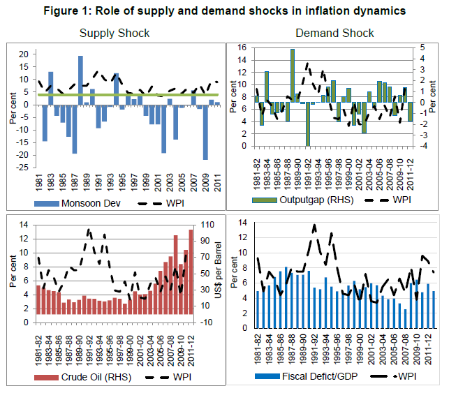

Although, the supply shocks are believed to have significant influence on inflation in India, the role of demand shocks, often originated through the dominance of fiscal deficit on monetary expansion during 1980s and 1990s, cannot be ignored. The automatic monetisation of government deficits fuelled inflationary pressures which in turn, created a wedge between government revenue and expenditure, thus, leading to a vicious nexus between fiscal deficits, money supply and inflation. Some of the phases of high fiscal deficit in the past have also witnessed a sharp rise in inflation. The monetary impact of fiscal deficit remained as one of the major concerns for monetary authority in 1990s. The high real growth and benign inflation experienced during the years 2003-04 to 2007-08 is often attributed to the policy makers’ efforts to ensure monetary and fiscal coordination with emphasis on fiscal prudence. In this context, the enactment of Fiscal Responsibility Budget Management (FRBM) act had also coincided with benign inflation trends.

The south-west monsoon has always played a vital role in determining inflation trajectory over the years. Large part of the country receives major rainfall during July-September that provides important source of irrigation for Kharif season. Although the impact of monsoon on agricultural production is limited thanks to the improvement in the technology used in irrigation, deficient monsoon continues to be a major factor tends to cause spikes in inflation. During the last three decades, the deficient monsoon (deviation from normal index) often resulted in sharp rise in inflation above the tolerable level of 4-5 per cent in India.

Against these backdrops, the present study makes an attempt to examine the role of demand and supply shocks in determining the inflation dynamics taking cognizance of the severe criticism leveled against the use of conventional measures of relative price shocks such as food and fuel inflation. We chose the standard Phillips curve framework and the P-star approach for examining the role of demand and supply shocks in determining the dynamics of inflation. The P-star model of inflation is considered as an alternative to the conventional Philips curve approach as the latter uses output gap as a proxy measure of demand shocks which are likely to contain significant measurement errors (Callen and Chang, 1999 and Nachane and Lakshmi, 2002). On the other hand, P-star approach uses money gap in lieu of output gap, which is theoretically more appealing and empirically well established in the literature. In addition, this study makes an attempt to construct a measure of supply shock which is free from any arbitrary selection of commodity prices or trimming of prices which appear on both tails of the distribution of commodity prices.

In order to analyse the dynamic impact of demand and supply shocks on inflation, we used vector autoregression (VAR) framework and estimated both the conventional time invariant and a time varying VAR models. The inferences concerning the dynamic response of inflation to shocks are drawn from impulse responses and decomposition of forecast error variances. The evidences from the impulse response of inflation to shocks in various supply shock measures suggested that the magnitude of inflation response is relatively larger to skewness based supply shock measure and the response is found to be more persistent if real money gap is used in the model as a proxy for demand shocks. Similarly, the response of inflation to real money gap is found to be much stronger as compared to output gap. The evidence with respect to the response of inflation to both demand and supply shocks indicated that the response of inflation to shocks is noticeably larger during the episodes of global financial crises.

The evidence with respect to inflation forecast error variance decomposition is consistent with what we had observed from the impulse response analysis. The skewness based supply shock measure is found to explain a significant portion of inflation forecast error variance as compared to the conventional measures such food and fuel inflation. The cyclical component of real money stock as compared to that of real output seems to have explained larger variation in inflation. In sum, the empirical evidence obtained from alternative econometric models consistently signifies the importance of both demand and supply shocks in explaining the dynamics of inflation in India.

The study is organised as follows. Introduction of the study is followed by section 2 which provides the theoretical approach for modelling inflation. The various methodologies used in construction of supply shocks are presented in section 3. Section 4 discusses the empirical findings of the study, while section 5 summarises the observations and findings of the study.

2. Theoretical Approach for Modelling Inflation

Although theoretical developments in this respect provide a number of alternative approaches to model inflation, we have focused on two prominent approaches which are popular in policy discourse: Quantity theory based P-star model and the New Keynesian Phillips curve. The new Keynesian version of Philips curve became prominent since 1990s and is considered to be the standard benchmark for modelling inflation. The standard new Keynesian Phillips curve specifies inflation as a function of expected inflation and excess demand or marginal cost measured by output gap, unemployment rate etc. The P-star approach has been derived from Quantity theory of money and it links the short run dynamics of observed inflation to the determinants of long run equilibrium inflation.

2.1 The New Keynesian Phillips Curve

The new Keynesian Philips curve is a modified version of Phillips curve introduced by Philips (1958). Earlier versions of Phillips curve postulate that there exists a stable trade-off between (wage or price) inflation and unemployment or output. Policy makers soon began to exploit the Philips relation which gave them a choice of lowering unemployment or increasing output at the cost of higher inflation and vice-versa. However, high rates of unemployment and inflation during 1970s were inconsistent with the Phillips relation. In this respect Phelps (1967) and Friedman (1968) argued that the trade-off between inflation and unemployment is not a permanent or long-run phenomenon.

Friedman-Phelps critique put forward two important propositions in modelling inflation: (i) it distinguished the relationship between inflation and output in the short-run and long-run; and (ii) it introduced the role of expectations in price adjustment process. The explicit role of expectations in the inflation dynamics carried the debate further on how the expectations can be formed. Phelps (1967) assumed adaptive expectation hypothesis in modelling expectations. Adaptive expectations assume that expectations are formed based on the past experience alone. Lucas (1972) and Sargent and Wallace (1975), however, argued that economic agents make expectations rationally and are capable of making accurate expectations taking all relevant information into account. Thus, rational expectations hypothesis implied that only unanticipated changes in the price level would affect output in the short run. In essence, the short run trade-off between output and prices arise due to misperceptions or imperfect information on the part of price setting agents (Lucas 1972).

The Lucas (1972) and Sargent and Wallace (1975) propositions were based on the assumption that prices adjust instantaneously to the departure of prices from its market clearing level. However, the available empirical evidences in favour of sluggish price adjustment as observed by Gordon (1976) undermine their arguments. Indeed, the role of supply shocks gained importance in predicting inflation during the 1970s. Accordingly, Gordon (1977, 1982) extended the expectation augmented Phillips curve by incorporating supply shocks, which is now popularly known as the “triangle” model. As the name suggests, the triangle model characterize the inflationary process on inertia, demand pressure and supply shocks. The empirical version of the triangle model of inflation (π_t) is: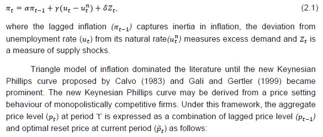

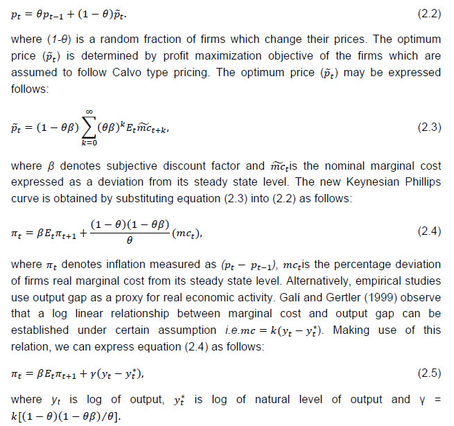Thus, the new Keynesian Phillips curve incorporates price rigidities into the model while retaining the assumption of rational expectation, which is forward looking. Consequently, the inflation is assumed to depend on current and future economic conditions alone (Clarida et al., 1999). However, empirical studies often report that output gap leads inflation which contradicts the theoretical proposition. In this respect, Galí and Getler (1999) proposed a ‘hybrid new Keynesian Phillips curve’ including a lagged inflation implying θ fraction of firms are backward looking while setting the price. The hybrid version of new Keynesian Philips curve is expressed as: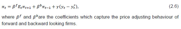

Due to its lucid micro theoretic foundations, large number of empirical studies attempted to establish this relationship using the data from various countries. Although, by and large the empirical studies from the developed countries supported this relationship, the evidence from developing countries seems to be mixed. In the literature, number of empirical studies from developing countries has failed to establish the short run association between output and inflation as predicted by the theory. Similarly, the forward looking term in the hybrid version of new Keynesian models was found to play very limited role in explaining inflation dynamics (Rudd and Whelan, 2005). Nonetheless, the new Keynesian models have contributed significantly in understanding inflation dynamics and are widely used in empirical studies.

2.2 The P –Star Models

The P-star approach, first proposed by Hallman et al. (1991), is based on the quantity theory of money. Under this approach, the short run fluctuations in inflation are attributed to the determinants of long run equilibrium price. Theoretically, the long run equilibrium price (p*) is determined by current money supply, potential income and the equilibrium velocity. In this framework, the actual aggregate price is assumed to adjust to its deviation from equilibrium level. In other words, it predicts that the actual price will rise, fall or remain unchanged depending on if the actual price is below, above or equal to its equilibrium level, respectively.

The traditional quantity theory relation is given as follows:

MV=PY,                                                                                      (2.7)

where M is stock of money, V is income velocity of money, P is aggregate price level and Y is real output.

The long run equilibrium price for a given the stock of money, the level of potential real output (Y*) and long run equilibrium value of velocity (V*) can be specified as follows:

Alternatively, in log form, equation (2.7) and (2.8) can be written as:

p = m + v - y,                                                                                     (2.9)

p* = m + v* - y*.                                                                                (2.10)

Equation (2.10) states that equilibrium price is equal to money per unit of potential output at equilibrium velocity (Tödter and Reimers 1994).

By subtracting equation (2.10) from (2.9), we can express the deviation of actual price from its equilibrium level in terms of velocity gap and output gap as follows:

(p - p*) = (v - v* ) - (y - y*).                                                                  (2.11)

Hence, by substituting price gap with real money gap in equation (2.12), we can arrive at equation (2.14). The readily available high frequency data on money supply makes such specification more amenable to empirical analysis. Moreover, the advantage of estimating the P-star model in terms of real money gap establishes a direct link between money and inflation as emphasised by the quantity theory. It can be easily shown that the P-star specification augmented by supply shocks is equivalent to estimating the new Keynesian Philips curve as given in equation (2.5) (Gerlach and Svensson, 2003).

3. The Methodology of Constructing Supply Shocks

The empirical examination of the dynamic link between relative price shocks and inflation crucially hinges on an appropriate measure of shocks. The empirical studies, at large, used an index of prices, which are highly volatile, as a measure of supply shocks and often believed to be outside the domain of the monetary authority. In this respect, constructs of food and fuel inflation are largely acknowledged as highly volatile components of aggregate inflation; hence, widely used as a proxy for supply shocks. In this context, there are broadly three different approaches available in the literature to measure supply shocks: exclusion method; limited influence method; and model based approach³.

Under exclusion method, certain prices are chosen as they are believed, in the perception of researchers, to be highly volatile items and constructs of such excluded items served as measures of supply shocks. This approach is widely followed, especially by the policy makers, as it is easy to construct and communicate. In this respect, use of oil prices as a proxy of supply shocks has become more relevant and popular after the episodes of oil price shocks in 1970s. Following the seminal work of Lucas (1973), there is voluminous empirical studies focused on the empirical relationship between such relative price shocks and inflation.

In a pioneering study, Bruno and Sachs (1985) have documented the effects of oil price shocks of the 1970s on output and inflation for major industrialized countries. Since then number of studies have used oil price as a measure of supply shock. Hooker (2002) examined the changing weight of oil prices as an explanatory variable in a traditional Phillips curve specification for the U.S. economy. Hamilton (2003) developed an index of dummy based on oil supply disruptions associated with major political crises experienced by oil-producing countries and investigated how well such index predicts oil prices and real GDP of U.S. A recent study by Ball et al. (2015) observed significant changes in food and energy prices and found that such relative price shocks seem to have influenced headline inflation, which in turn affected expected inflation and future core inflation⁴.

The limited influence method proposed by Bryan and Cecchetti (1993) involves trimming of certain percentage of prices on both extremes of the distribution of price changes to arrive at a measure of core inflation. The commodity prices which are trimmed out are considered as supply shocks. The advantage of this procedure over the exclusion method is that the set of commodity prices eliminated in each period varies over time. However, trimming certain percentage of prices symmetrically on both tails of the distribution is appropriate if and only if the distribution of commodity prices is symmetric. In reality, however, the cross sectional distribution of commodity prices is often found to be skewed; hence, symmetric trimming tends to produce an element of error in the measurement of supply shocks.

Against this background, Roger (1997) proposed a method that determines the percentage of trimming for each tail of the distribution based on the sign of skewness. More specifically, in case of positively skewed distribution of price changes, the procedure suggests that the trimming percentage is to be centered to the right of the 50th percentile of the distribution. However, the core inflation measure obtained from such asymmetric trimming depends on the choice of the trimming percentage and the percentile center considered. In order to resolve this issue, Kearns (1998) and Meyler (1999) define an optimal size of trimming that ensures a measure of core inflation lying closer to the reference trend component of inflation. However, core inflation so obtained is again conditional upon the selection of the reference trend inflation.

There are some efforts to construct measures of supply and demand shocks by imposing theoretical restrictions on the parameters of the econometric models. The empirical studies largely depend on structural vector autoregression (SVAR) models and impose structural restrictions to identify demand and supply shocks. There are two broad approaches available for identi­fication of structural supply and demand shocks in the literature. These include the SVARs proposed by Blanchard and Quah (1989) and identifi­cation by sign restrictions on the impulse responses proposed by Uhlig (2005). The study by Blanchard and Quah (1989) provides an identification scheme of long run restriction which helps in measuring the role of demand and supply shocks. On the other hand, sign restrictions are imposed on the parameters of the VAR model to identify the positive/negative relationship among demand and supply shocks. These restrictions provide impulse responses that are consistent with standard theoretical predictions.

The study by Cashin et al. (2012) found that frequent changes in oil prices, which are largely considered as exogenous shocks, have an asymmetric impact on inflation depending on whether changes in oil price is driven by supply or demand shocks. The study found that almost all countries under consideration experienced long-run inflationary pressure in response to demand shock induced oil price rise and the impact of such demand shocks seem to have short lived on real output. On the contrary, a supply shock induced oil price rise is found to have long lasting adverse impact on growth while inflation response to such adverse supply shocks seems to have short lived. These evidences suggest that even if demand and supply shocks are normally distributed the resulting distribution of growth is likely to be negatively skewed.

In the recent times, the application of dynamic stochastic general equilibrium (DSGE) framework gained significance in empirical literature and there are few studies which apply this framework to examine the dynamics of inflation in response to supply and demand shocks. The DSGE models impute the supply and demand shocks into the structural equations in number of ways through changing the structural coefficients. In this context, Dées et al. (2010) estimated a multi-country version of the standard DSGE New Keynesian (NK) model using IS curve, Phillips curve and standard Taylor Rule for measuring the impact of demand and supply shocks in the economy. The study found that impact of supply shocks account for nearly all the variation of inflation in the short run, but the impact declines rapidly and account for about half of the variation of inflation in the long-run. Thus, the empirical studies largely document evidences to support the importance of demand and supply shocks on inflation. Moreover, the exogenous supply shocks seem to have played a significant role in determining the magnitude of inflation and its persistence.

Although the measures of supply shocks obtained through exclusion method is easy to construct and communicate, use of such measures in applications attracted severe criticism. It is often criticized on the ground that it involves a great deal of arbitrariness in choosing the commodity prices to construct the measure of supply shock. The limited influence method, as it is mentioned elsewhere in this study, also suffers from the criticism of arbitrary selection of trimming percentage. The measures obtained from theoretical models using econometric tools seem to be theoretically more appealing. However, the supply shock measures are obtained by imposing structural restrictions on the parameters of the econometric models. The structural restrictions are generally decided by the theory and hence, a construct of supply shocks is conditional upon the choice of the theoretical framework that the researcher chooses. Since there are always competing theories to explain a particular phenomenon, the measure of supply shock obtained utilizing a particular theoretical model turns out to be a choice among the possible alternative measures.

Taking cognizance of these issues, the present study depends upon the methodology recently introduced by Rather, Durai and Ramachandran (2016) to construct a measure of supply shocks. This approach mainly focuses on constructing core inflation by eliminating a set of commodity prices through an optimizing mechanism in such a way that the cross sectional distribution of remaining prices has symmetric distribution. In other words, a set of prices are eliminated from all the possible combination of cross sectional prices for every time period to minimize the skewness of remaining prices. The commodity prices so excluded are used to construct measures of supply shocks. Under this approach, therefore, the choice of commodities as well as the number of commodity prices to be considered for elimination might vary every time period. Therefore, this method does not involve any arbitrary selection of commodity prices or trimming percentage to construct an index of supply shock measure.

This approach mainly involves construction of core inflation by subtracting transitory elements from measured inflation. In this context, Ball and Mankiw (1995) provide a theoretical rationale for a temporary deviation of inflation (π) from its underlying trend (π^c). They consider an economy that contains a gamut of industries, each with a set of imperfectly competitive firms. Assume that the desired price change of an industry is π^c + θ in a given period, where π^c is price change common across all industries, mainly determined by the monetary pressure in an economy, and θ is the price change originating from idiosyncratic shocks which follows skew-normal distribution with zero mean and probability density function f(θ). In the presence of menu cost (C), with cumulative distribution function G(.), the actual price change for each industry is π^c+{(θ) G(|θ|)}; where π^c is the common price change which is fully effected across all industries and (θ) G(|θ|) is the actual price change in response to θ. Note that the actual change in price {(θ) G(|θ|)} differs from θ as not all the firms adjust prices in the presence of the menu cost. The realized aggregate inflation is:

Thus, if the density of shocks f(θ) is symmetric {f(θ)=f(-θ)} then the observed inflation (π) is the same as its underlying trend (π^c). On the contrary, if f(θ) is skewed {f(θ)≠ f(-θ)} then observed inflation (π) differs from π^c. Based on this premise, we minimize the skewness of actual price change π^c+{(θ) G(|θ|)} as it would minimize the influence of θ on π and uncover π^c; a common component of price changes across all commodities.⁵

Therefore, the trimming percentage and the extent of trim for each tail of distribution for each time period is endogenously and uniquely determined based on the magnitude and sign of its skewness for the corresponding period. Hence, unlike conventional trimmed mean approach, the trimming percentage under this approach varies over time.

4. The Empirical Analysis

The empirical investigation focuses on two important issues: (i) whether impact of supply shocks on inflation is significant and lasting for a longer period; and (ii) what is the relative importance of real output gap and real money gap in explaining the dynamics of inflation. The empirical estimation is conducted using monthly time series data from January 2005 to September 2014. We confine to this sample period for the reason that consistent time series data on gross domestic product at constant price based on 2004-05 prices is available up to second quarter of 2014-15⁶. Three alternative measures of supply shocks based on exclusion method, trimmed mean method and based on the methodology presented in section 3 are used in the estimation. The measure of money gap is obtained by taking the deviation of real M3 money stock from its long term trend defined as Hodrick-Prescott filter. The deviation of real GDP at factor cost from its Hodrick-Prescott trend is used as a measure of output gap. The inflation is measured as monthly percentage change in wholesale price index.

4.1 The GMM estimates

First, we estimate the following econometric specifications derived from the theoretical frameworks of Phillips curve and P-star models:

We consider two lags of inflation as explanatory variables in both equations as lags beyond two are found to be statistically insignificant.

To begin with, the equations are estimated using generalized method of moments (GMM) and the instruments used in the estimation include a constant, third to sixth lags of inflation, five lags of either output gap or real money gap and five lags of supply shocks. The heteroscedasticity and autocorrelation consistent covariance matrix of coefficients are obtained using Newey-West method and weights are updated continuously till convergence is achieved. Since there are fifteen instruments and only five parameters to be estimated, the model is over-identified; hence, it is necessary to examine whether the over-identifying restrictions are binding on the results. In this respect, we have used the J-statistic that follows X² distribution to test the null hypothesis that over-identifying restrictions are not binding.

The estimates of equations (4.3) to (4.8) labelled as Model 1 to 6 are presented in Table 1. The probability value associated with J-statistic for each of the estimated model shown in the last row of Table 1 are above 0.05, confirming that the over-identifying restrictions are not binding.

The parameter estimates of the models indicate that coefficient with respect to first lag of inflation is statistically significant only in model 1 and model 4 whereas none of the coefficients associated with the second lag is significant. The coefficient with respect to output gap is positive and significant only in model 2. Further, money gap is found to be significantly impacting inflation in a positive direction in models 4 and 5. The coefficients with respect to measures of supply shocks are also positive and statistically significant in all models excepting model 2. These evidences are intuitively more appealing in the sense that output gap, money gap and supply shocks do significantly contribute to inflation positively.

Further, we compare the out of sample forecast performance of these competing models using Diebold and Mariano predictive accuracy tests. This exercise has been carried out to understand whether money gap has additional information content as compared to output gap in predicting future inflation. In addition, it helps in assessing relative predictive accuracy of different models containing alternate measures of supply shocks. The Diebold-Mariano (DM) statistics obtained from the Mean square error (MSE) of the estimated models as indicated in parenthesis is used to examine the predictive accuracy and the results are presented in Table 2. We note that model 4 has the least MSE and the probability values associated with DM test statistic proves that model 4 is significantly different from all other models in predicting inflation. These evidences confirm that model 4 which contains real money gap as demand shock and deviation of actual inflation from core inflation as supply shock has additional information content as compared to all other models in predicting inflation.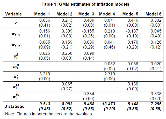

4.2 The Vector Autoregression (VAR) Analysis

In this section, we consider a three variables VAR model and mainly focus on the dynamic response of inflation to demand and supply shocks. The variables are chosen either based on the Phillips curve relationship or the P - star model presented in section 2. The variables in the VAR model are ordered as supply shock, demand shock and inflation. The data are pretested for their time series properties using a battery of unit root tests and the results suggested that they are stationary process¹⁰.

It is evident that the response of inflation to shocks in real money gap is much more than the shocks in real output gap. Hence, the p-star model which includes real money gap as the measure of demand shock is found to be more appropriate in explaining the dynamics of inflation than the standard Phillips curve model consisting of real output gap as the measure of demand shock.

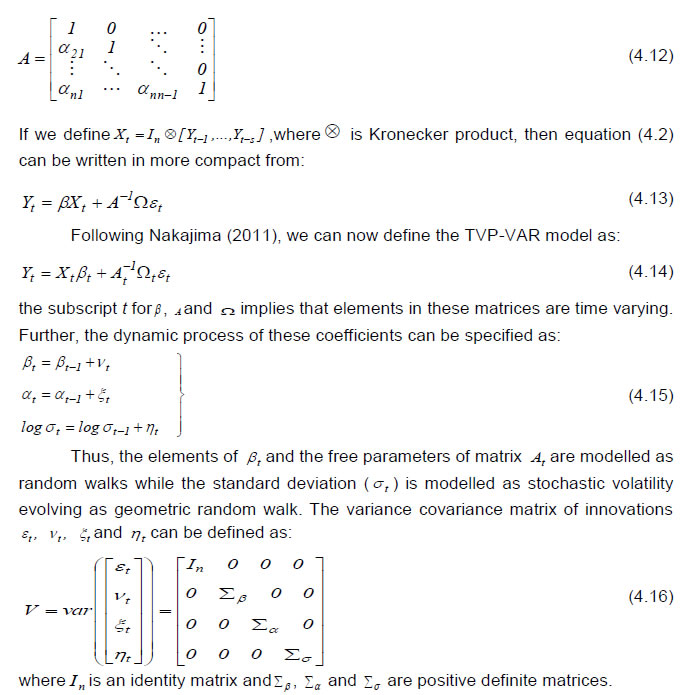
Further, we present in Table 3 and 4 the forecast error variance decomposition of inflation due to supply shocks and demand shocks respectively at different forecast horizons. We did not proceed beyond twelve months forecast horizon, because there was no change in proportion of variance explained by different shocks; suggesting that the dynamic impact of both supply shocks and demand shocks on inflation forecast persists for a maximum of twelve months and even less in some cases.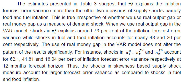

The results concerning the decomposition of forecast error variance of inflation with respect to demand shocks are presented in Table 4. This exercise is basically to capture the relative importance of real output gap and real money gap in explaining the forecast error variance of inflation. One major inference emanates from the Table is that shocks in real money gap explains relatively larger variance in inflation forecast errors. This result is robust irrespective of various measures of supply shocks used in the VAR model. This evidence signifies the fact that real money gap has an edge over real output gap in explaining the inflation dynamics.

4.3 Time Varying Parameter VAR Model

Although evidences obtained from GMM estimates, impulse responses and variance decomposition invariably support the view that the real money gap explains the dynamics of inflation better than real output gap, certain empirical results are not very convincing on the theoretical grounds. For instance, the impulse responses obtained from the VAR model indicate that inflation responds negatively to adverse supply shocks. This may be due to breaks in the dynamics between inflation and supply shocks or in other words the dynamics might have undergone a change during the sample period. Under such circumstances, estimating inflation models assuming constant parameters over the sample period is likely to produce misleading inferences.

Moreover, it is widely acknowledged that the underlying structural relationships among variables are most likely to vary over time; hence, the conventional approach of assuming parameter constancy while estimating time series econometric models seems to be implausible. In addition, the data generating process of economic variables, at large, seem to have a drift and the volatility process may not be time invariant. If this is the case, econometric models which assume constant parameter and time invariant volatility tend to produce inconsistent and inefficient estimates (Nakajima, 2011). In this context, the time varying parameter vector autoregression model (TVP-VAR) model introduced by Primiceri (2005) appears to be a better option as it allows the coefficients to vary over time and captures the shocks in volatility. Under this approach, the parameters of the VAR model are generally assumed to follow a first order random walk process; hence, it automatically tracks temporary or permanent shift, if any, in the parameters of the model.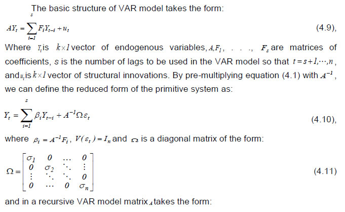

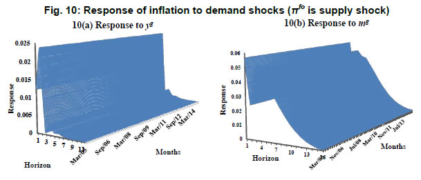
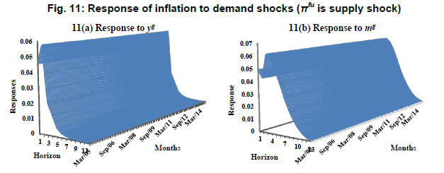
Following the baseline specification of time invariant VAR, we estimate a TVP-VAR model with the same set of variables and ordering structure. The lag length used in this case is also two in order to maintain uniformity in specification. The estimation of TVP- VAR model is done under a Bayesian approach using Markov Chain Monte Carlo (MCMC) method which provides precise and efficient estimation. For this purpose, as generally practiced in the literature, the Gibbs sampler is employed to implement the MCMC algorithm in our present study as well. Following Nakajima (2011), we setup our estimation procedure with reasonably flat priors for the initial state of parameters. The hyper parameters for the i_th diagonal element of the covariance matrix are set as indicated in Table 5:

For other parameters of the model, the priors are set as: μ_β0=μ_α0=μ_σ0=0. The posterior estimates are obtained using MCMC method by drawing 10,000 samples after initial 1,000 samples were discarded in the burns-in.

The convergence diagnostic statistics (CD) of Geweke (1992) and inefficiency factors of selected parameters computed using MCMC sample are reported in Table 6. The results indicate that based on the value of CD statistic the null hypothesis of convergence to the posterior distribution cannot be rejected at 5 per cent level of significance. The inefficiency factors are also found to be quite low for the parameters. These results indicate that the selected sampling method efficiently produces samples with low autocorrelation.

The analysis of impulse response functions in the TVP-VAR framework has an edge over the time invariant VAR model as in the former case we can analyse the response of variables to a given shock at every point of time over the entire sample period. The magnitude of impulse given to variables is equal to the average stochastic volatility of the given variable during the entire sample period. This methodology also has an advantage of presenting the impulse response coefficients in the form of three dimensional charts as presented in Fig. 7 to 11. The X-axis shows the sample range, Y-axis represents the time horizon and Z-axis measures the impulse response. Hence, we can track the response of variables to a given shock at different time horizons over the entire sample period which will facilitate the analysis of responses over both short run (lower time horizons) and long run (higher time horizons) over the entire sample period.

The impulse response of inflation to the alternative measures of supply shocks obtained from Phillips curve relationships and the P-star model are presented in Fig. 7 and 8 respectively. The response of inflation to a shock in π^s presented in Fig. 7 (a) shows that inflation responds positively to shocks in π^s. The impact of π^s on inflation is observed to be significantly positive upto a period of twelve months with the responses decaying out slowly after reaching its peak in the first month. From the magnitude of impulse responses over the sample period, we note that the response of inflation to shocks in π^s are found to be larger from the first quarter of 2007-08 till the mid of 2012-13. Moreover, we also note that the responses are increasing in their magnitude in the recent time periods.

The response of inflation to shocks in π^fo is produced in Fig. 7 (b). It is evident that the response of inflation to shocks in food inflation is positive throughout the sample period. The impact of food inflation on inflation was at its peak in November 2009. Moreover, a twelve month time horizon shows that the magnitude of response of inflation to shocks in π^fo increases till the third month following which they decline by twelfth month. Finally, the response of inflation to shocks in π^fu seems to be similar to what we had witnessed with respect the response of inflation to shocks in π^s. The magnitude of impulse response declines after the first month and remains significantly above zero for less than twelve months. In this case, we also observe that the variations in the response of inflation over the sample range is observed only upto sixth months ahead horizon following which the responses do not exhibit fluctuations over time. The response of inflation seems to be weakening in the recent periods as observed in Fig. 7(b). On the whole, we observe that among the three alternate measures of supply shocks, shocks in π^s are found to be having relatively large impact on inflation, which is, at large, consistent with the evidence obtained from GMM estimates and constant parameter VAR models. These evidences suggest that measures of supply shocks obtained from the methodology proposed by Rather, Durai and Ramachandran (2016) have played a significant role in the explaining the dynamics of inflation.

The impulse response coefficients of inflation to shocks in π^s, π^fo and π^fu obtained from P-star model in which money gap is used as measure of demand shock are shown in Fig. 8(a), (b) and (c) respectively. In Fig. 8(a) we observe that the response of inflation to shocks in π^s remain positive during the first two months and turn negative thereafter. The negative impact of shocks in π^s on inflation was also observed as in the case of time invariant parameter VAR model. Analysing the impulse responses over the sample range indicate that the magnitude of impact of shocks in π^s on inflation was high from the middle of 2007 till the end of 2012 and it further seems to stabilize, especially during the recent periods. The persistence of impact in this case was found to be more as compared to what we observe in Fig. 7(a) where the real output gap was used as the measure of demand shock.

The response of inflation to shocks in π^fo presented in Fig. 8(b) is found to be largely negative over the period of twenty months with the exception of second to fourth month. Further, the shocks in π^fo are observed to impact inflation much more till the end of 2011 than the recent periods during which it is relatively stable. The response of inflation to shocks in π^fu presented in Fig. 8(c) shows similar results as we had observed in Fig. 8(a) with an exception that the persistence of impact of shocks on inflation being less than what we had seen with the model based on the Phillips curve relationship. It is also observed that inflation responds positively to shocks in π^fu during the first two months and subsequently turns out to be negative for rest of the months. The response of inflation to fuel price shocks is relatively weaker during the initial sample period i.e. before 2007. Its magnitude increased noticeably during 2007 towards the end of 2011 and subsequently the impact remained stable.

The major findings that emerge from Fig. 7 and 8 are that the impact of shocks in π^s on inflation is found to be larger as compared to the other two traditionally used measures of supply shocks i.e. food inflation and fuel inflation. Moreover, the empirical evidence obtained from the model that has real money gap as a measure of demand shocks indicate that the response of inflation to shocks are highly persistent.

We have also observed that the response of inflation to supply shocks was considerably larger in magnitude during the period of 2007 to 2012; coinciding with the episodes of Global Financial Crisis and the Eurozone Crisis. This evidence is consistent with the findings of Patra et al. (2013) that the inflation persistence increased in the post global crisis period.

Further, we examine the impact of demand shocks on inflation and the relevant time varying impulse responses are being produced in Fig. 9, 10 and 11. The response of inflation to the two alternative measures of demand shocks i.e. real output gap (y^g) and real money gap (m^g) are presented in panel (a) and (b) respectively of Fig. 9, 10 and 11. In Fig. 9(a), we observe that the response of inflation to shocks in y^g is positive throughout the sample period and across the time horizon of twelve months. The maximum impact is observed in the second month, following which the responses remain stable during third and fourth month and decline thereafter. The variations in responses over the sample range are found to be relatively stable for all time horizons except in the first month, which shows that the impact of shocks in y^g on inflation is increasing in the recent periods, especially after 2011. In the case of response of inflation to shocks in m^g presented in Fig. 9(b), the impact is maximum in the first month, falls by 50 per cent in the second month, but rises again in the third month and continues to decline thereafter. As far as changes in the responses over the sample range is concerned we note that the response remained stable prior to the mid of 2007 and after the end of 2012 with a sharp rise in the impact of shocks in m^g on inflation between 2007 and 2012. Moreover, we also notice that the response of inflation is more persistent and higher in magnitude to shocks in m^g than to shocks in y^g.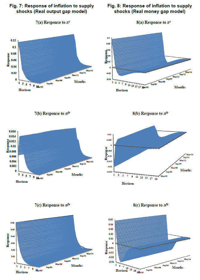

The plots in Fig. 10 are the response of inflation to shocks in y^g and m^g when food inflation is used as a measure of supply shock. In panel (a) of Fig. 10, we observe that the impact of shocks in y^g on inflation is positive and short lived. The response of inflation doubles in the second month as compared to first month and falls drastically in the third month. Further, trend in response of inflation over the sample range shows that inflationary impact of demand shocks increased in magnitude over time.

We now move on to analyse the response of inflation to shocks in m^g as presented in Fig. 10(b). The responses in this case bear resemblance to the previous case (Fig. 9) with respect to magnitude and persistence. The impact of shocks in m^g on inflation is observed to maximum in the first month and declines to less than half of it in the second month. There is a gradual decline in response from the fourth month onwards and reaches close to zero in the sixteenth month; indicating that there is long persistence in responses as compared to Fig. 10(a). In this case, the analysis of responses over the sample period shows different results in the short run and long run. In the short run i.e. up to three months horizon we observe that the responses show a downward trend indicating that the impact of shocks in m^g have gradually weakened over the years. However, as we move on to higher time horizons, we observe that the responses appear to be in an inverted U-shaped pattern with a flat tail towards the end of the sample period.

Finally, we examine the response of inflation to demand shocks when fuel inflation is used as a measure of supply shock and the relevant plots are produced in Fig. 11. The response of inflation to shocks in y^g presented in Fig. 11(a) is again found to be maximum in the second month following which it decreases sharply. An examination of the change in responses over the sample period reveals that the inflationary impact of shocks in y^g exhibit noticeable climb between the mid of 2009 and end of 2011, subsequent to which it declines. The response of inflation to shocks in m^g presented in Fig. 11(b) shows that the impact is maximum in the third month and persisted upto twelfth month. This is contrary to the previous cases presented in Fig. 9 and 10 in which we had observed that the responses are maximum in the first month and persist till sixteenth month. Nonetheless, the variations in responses over the sample period seem to mimic the patterns as observed in Fig. 9(b) in the sense that responses are relatively high during 2007 to 2012 and flatter otherwise, especially in the recent time periods.

In sum, the results concerning the response of inflation to demand shocks reveals that real money gap impacts inflation much more than real output gap in all the three cases. Additionally, the response persists more in the case of real money gap than in the case of real output gap. The analysis of responses over the sample range in all the three cases shows that the inflationary impact of demand shocks was relatively larger during 2007 to 2012. These results are very similar to those obtained in the case of impact of supply shocks on inflation, which leads to the conclusion that the role of shocks in driving inflation was significantly high during the crisis period and the impact of such shocks seems to have moderate impact on inflation in the recent time period.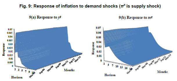

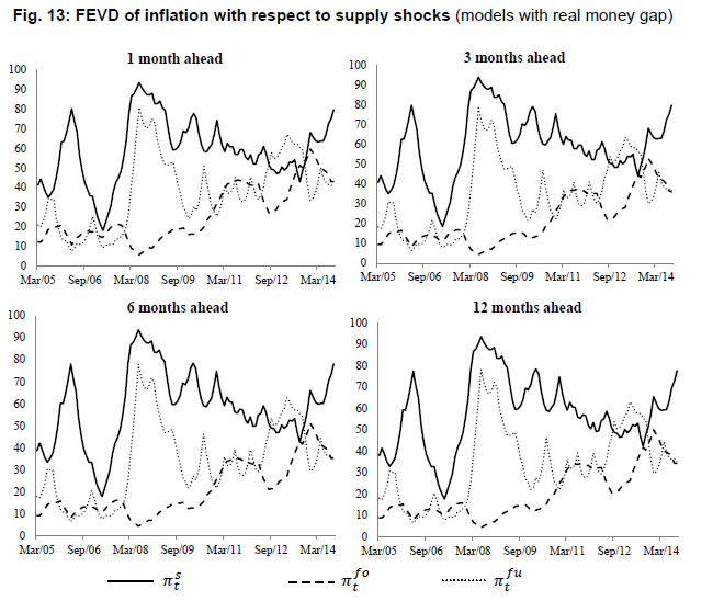
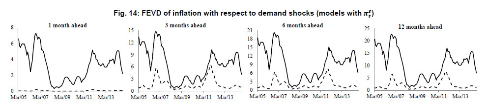
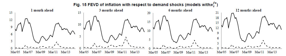
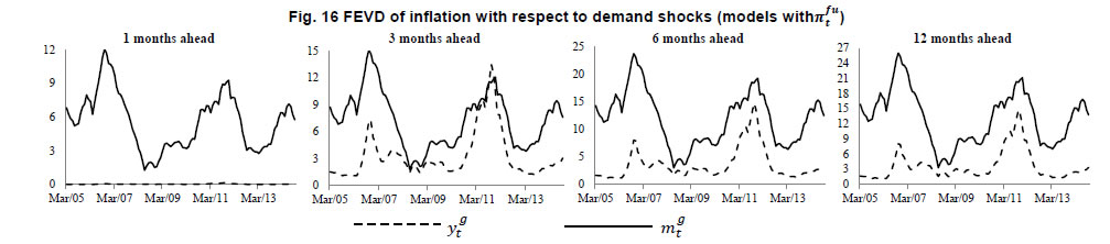
Apart from analysing the impulse response functions, we have examined the Forecast Error Variance Decomposition (FEVD) of inflation with respect to supply shocks and demand shocks using TVP-VAR framework. This gives us insights into the contribution of different shocks to variance in inflation over time. The FEVD of inflation in all the models have been derived at multiple time horizons (1 month, 3 months, 6 months and 12 months) and we have presented the plots of the same in Fig. 12 to 16.

The FEVD of inflation with respect to supply shocks when real output gap and real money gap are used as alternate measures of demand shocks are produced in Fig. 12 and 13 respectively. The plots of FEVD of inflation in Fig. 12 clearly indicate that shocks in π^s has maximum contribution to variance in inflation at all time horizons. This is followed by contributions from shocks in fuel inflation and food inflation respectively. The contribution of π^s to variance in inflation is at its peak of 92.3 per cent in August 2008 which coincided with the start of Global Financial Crisis. Another important point to be noted in this regard is that this peak was preceded by another peak of 81 per cent in April 2006 following which the contributions fell drastically to 15.7 per cent in April 2007 within a span of 12 months and rose again sharply till August 2008. Thus, we observe excessive fluctuation in the contribution of π^s to variation in inflation during the pre-crisis period. Following this episode, we observe a downward trend in the contribution of this shock till the second half of 2013, subsequent to which it again rose steeply towards the end of the sample period. Although shocks in π^s predominantly contributes to variance in inflation, the shocks in π^fu were found to contribute more than other supply shocks during some time period.

The FEVD of inflation presented in Fig. 13 is obtained from the model consisting the real money gap is used as a measure of demand shock. In this case also, we observe that the shocks in π^s contributes maximum to variance in inflation as compared to shocks in other two measures of supply shock. The maximum contribution of π^s is observed in July 2008 as in the previous case and there is, however, not much difference in the magnitude of contribution. In the subsequent time period, we do not observe any significant deviations in the patterns of contributions of supply shocks to variations in inflation as compared to what we have observed in Fig. 12. Thus, the inference from Fig. 12 and 13 suggest that the forecast error variance of inflation is largely explained by shocks in π^s followed by π^fu and π^fo respectively. The maximum contribution of π^s to variance in inflation was observed in the beginning of Global Financial Crisis in the year 2008.

Further, we analyse the FEVD of inflation with respect to demand shocks in Fig. 14, 15 and 16. The solid lines, which represent the contribution of real money gap, undoubtedly contribute more to variance in inflation as compared to real output gap indicated by dashed lines in all the three cases at different time horizons. The maximum contribution of m^g to variations in inflations is observed in November 2006 in Fig. 14 and 16 where we have used π^s and π^fu as measures of supply shock respectively. When we use π^fo in the model, the maximum contribution of m^g is observed in February 2007. Notice that there is a downward trend in the contributions of m^g towards the middle of 2008, following which it picks up again and reaches another peak by the last quarter of 2011-12. However, the proportion of variance influenced by m^g declined drastically towards the end of the sample period. The contribution of shocks in real output gap (y^g) to the variance in inflation is almost negligible except in Fig. 16 where we have used fuel inflation as the measure of supply shock, excepting at higher time horizons. On the whole, we observe that the contribution of shocks in both m^g and y^g to inflation forecast variance has similar pattern across all the forecast time horizons. However, shocks in m^g has relatively larger influence as compared to shocks in y^g on the variance of inflation. Thus, the evidence obtained from the decomposition of forecast error variance unambiguously suggests that the P-star model explains the dynamics of inflation much better than the model based on Phillips curve relationship. These results derived from the TVP-VAR framework, at large, corroborate those evidences obtained from the time invariant parameter VAR model.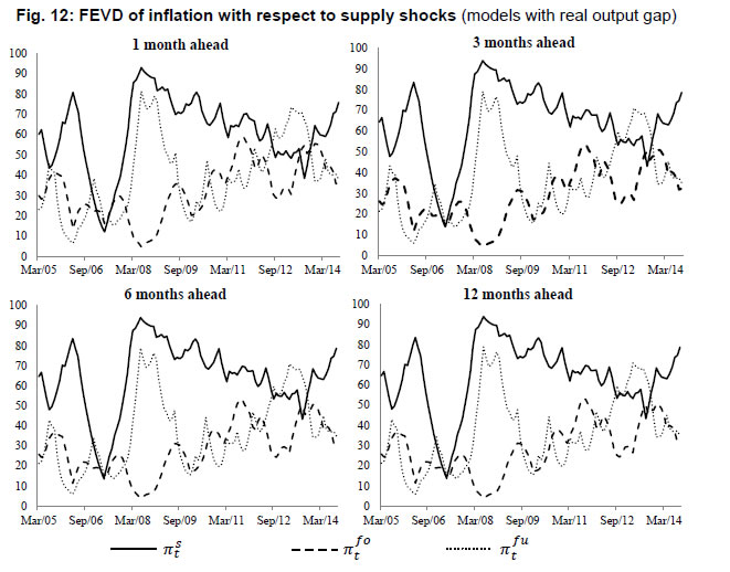

5. Conclusion

The aim of this study is to undertake an in-depth analysis of how shocks from both demand side as well as from supply side factors influence the dynamics of inflation in India. In this context, we have considered two measures of demand shocks viz. real output gap (y^g) and real money gap (m^g) and three measures of supply shocks viz. deviation of actual inflation from core inflation (π^s), food inflation (π^fo) and fuel inflation (π^fu). The real output gap and real money gap have been calculated as the deviation of real GDP and real M3 money stock respectively from their long run trend defined as their Hodrick-Prescott filter. Further, the calculation of π^s involves obtaining a measure of core inflation. This study replicated the recently introduced methodology of Rather, Durai and Ramachandran (2016) to construct the measure of core inflation and the measure of supply shock is then obtained by subtracting core inflation from headline inflation. The supply shocks are measured as monthly percentage change in respective price indices viz., food and fuel items of wholesale price index and index of prices that causes skewness in the cross-sectional distribution of individual commodity prices. The empirical estimation is conducted using monthly time series data from January 2005 to September 2014. The sample period is suggested by the availability of consistent time series data on real GDP and commodity-wise price indices.

The empirical investigation focuses on two important issues: (i) whether the impact of supply shocks on inflation is significant and persistent for a longer period; and (ii) whether the cyclical components of real GDP or real money stock performs better in explaining the dynamic of inflation. In addition, alternative measures of supply shocks are used in both models to evaluate whether methodologically sophisticated measure has an edge over the widely used conventional measures of supply shocks in explaining the dynamics of inflation. To this end, the present study utilizes the Phillips curve relation and P-star specification to model the inflation.

Three alternative econometric tools have been used to estimate the inflation models mainly to examine the robustness of the results. First, we have estimated the inflation equations using the generalised method of moments and used the predictive accuracy tests to determine the relative performance of the chosen models. Second, the conventional vector autoregression models are estimated mainly to obtain the impulse responses and decomposition of forecast error variance of the inflation, as it would help in understanding the dynamics of inflation. Third, a time varying vector autoregression model is estimated under the presumption that the dynamic relationship between inflation and its prime determinants might have undergone a structural change.

The evidence derived from the GMM estimates support the P-star model against the use of Phillips curve based model to explain the inflation dynamics; the coefficients with respect to both shocks in the P-star model are positive and highly significant. The magnitude of these coefficients in the P-star model is found to be relatively larger as compared to the corresponding coefficients obtained from the Phillips curve based equation. Among the competing specifications, the Diebold and Mariano predictive accuracy tests suggest that the inflation equation having the cyclical components of real money stock and the skewness based supply shock measure performs better in predicting inflation as compared to other specifications.

Subsequently, in order to examine the relative impact of demand and supply shocks and their persistence on inflation, we have constructed six different variants of a three variable VAR model consisting of inflation and measures of demand and supply shocks. The evidences from the impulse response of inflation suggest: (i) the magnitude of inflation response is relatively larger to shocks in skewness based supply shock measure; (ii) such response is found to be more persistent when we use the real money gap as a measure of demand shock; and (iii) the response of inflation to demand shocks measured as money gap is relatively stronger. Thus, the results from the conventional vector autoregression model suggest that the P-star model has an edge over the model ascribed by Phillips curve relationship in explains the dynamics of inflation and these results are largely in conformity with the evidence obtained from generalised method of moments estimates.

The inference from the forecast error variance decomposition of inflation due to supply shocks and demand shocks at different forecast horizons seems to favour the use of money gap and skewness based supply shock measures in the inflation model. For instance, the skewness based supply shock measure explains around 73 per cent of inflation forecast variance whereas the conventional measures i.e. food inflation and fuel inflation explains around 25 and 46 per cent, respectively. Further, money gap has larger contribution as compared to output gap to the variation in inflation forecast variance. Thus, the evidence from the conventional vector autoregression models signifies the fact that the supply shock measured as skewness of price distribution and cyclical fluctuations in real M3 money stock have an edge over their counterpart measures in explaining the inflation dynamics.

The major contribution of this study lies in the use of a time varying vector autoregression framework to understand the dynamics of inflation over time. The evidence from both time varying impulse responses and decomposition of inflation forecast variance suggests that the dynamics of inflation during the sample period has undergone significant change. An examination of impulse responses reveals that inflation response to demand as well as supply shocks is found to noticeably larger in times of global financial crises and Euro zone crises that occurred during the years 2007 to 2012. In conformity with the evidence obtained from GMM and time invariant vector autoregression estimates, the time varying model also suggests that real money gap and supply shock measure defined as skewness of cross sectional price distribution stand out as better candidates in explaining the inflation dynamics.

The empirical evidence obtained from alternative econometric models consistently signifies the importance of both demand and supply shocks in explaining the dynamics of inflation in India. The researcher must pay adequate attention on the methodology used in the construction of variables such as measures of demand as well as supply shocks, because the impact of alternative measures of such variables on inflation significantly differs. Moreover, the use of conventional time invariant econometric models may not be appropriate in capturing the behaviour of inflation, as the factors affecting inflation seem to have undergone significant change over time.

¹ M. Ramachandran (ramachandraneco@gmail.com) is presently Professor in the Pondicherry University, Pondicherry; while Rakesh Kumar (rarya@rbi.org.in) is Assistant Adviser in the Department of Economic and Policy Research, RBI. The views expressed in this Study are those of the authors.

² Darbha and Patel (2012) find that inflation is largely cross-sectionally diffused and driven by increasingly persistent common factors in non-food and non-energy sectors compared to that in the 1990s. On the contrary, the study by Patra et al. (2013) documents evidences to show that relative price shocks, mainly attributed to rise in food prices, caused positive skewness in the cross sectional distribution of prices, which in turn influenced general prices.

³ The construct of supply shocks is generally obtained by subtracting the underlying inflation from the headline inflation and hence, effort is directed to identify the underlying inflation or the core inflation so that the remaining component of headline inflation can be considered as a measure of supply shocks. For a brief review on the methodology of constructing core inflation see Bryan and Cecchetti (1993), Roger (1997), Wynne (1999), Meyler (1999), Marques and Mota (2000), Bagliano and Morana (2003).

⁴ There are empirical studies which consider global commodity prices as an indicator of supply shocks to examine their role in monetary policy transmission (Romer and Romer, 2004). Dua and Gaur (2010) in a multi country study found that global oil price shocks had significantly influenced aggregate inflation. Bhanumurthy et al. (2013) report that in the year of oil price shock when there is no pass-through inflation does not rise as it is being absorbed by policy but growth declined. In case of partial pass-through, a 10 per cent rise in oil price increases inflation by 0.3 per cent while there is full pass-through inflation increases by 0.6 per cent.

⁵ This method has a limitation when the skewness associated with the distribution of idiosyncratic shock is constant over time in the sense that the measure of core inflation (π^c) will be poor measure of underlying inflation; hence a poor predictor of headline inflation as well. However, the empirical evidence across countries shows that the measure of skewness varies significantly over time (see e.g., Ball and Mankiw, 1995; Kearns, 1998; Marques and Mota 2000; Pou and Debus, 2008; Rather et. at., 2015). For India, the estimate of standard deviation of skewness for the sample period is 1.37; implying a significant variation in the skewness over time.

⁶ Subsequent to Q2 of 2014-15, data on GDPFC at constant prices is available as Gross Value Added based on 2011-12 prices which is not consistent with the previous definition. Monthly time series data on real GDP at factor cost is obtained by interpolating the quarterly data using the methodology of Chow and Lin (1971) and monthly data on index of industrial production is used as the related series.

⁷ The derivation of these equations with a brief theoretical background for the respective equations are presented in section 2.

⁸ Core inflation is calculated based on the methodology proposed by Rather, Durai and Ramachandran (2016) as mentioned in section 3.

⁹ Food inflation and fuel inflation are measured as monthly change in the wholesale price indices of ‘food articles’ and ‘fuel and power’ respectively.

¹⁰ The unit root tests results are not produced to preserve space and it can be obtained upon request from the authors.

References

Ball, L. and N. G. Mankiw. 1995. “Relative-Price Changes as Aggregate Supply Shocks.” The Quarterly Journal of Economics 110(1): 161-193.

Ball, L., A. Chari and P. Mishra. 2015. “Understanding Inflation in India”. NBER Working Paper No. 22948.

Bagliano, F.C. and C. Morana. 2003. “Measuring US Core Inflation: A Common Trends Approach.” Journal of Macroeconomics 25(2): 197-212.

Bhanumurthy, N. R., S. Das and S. Bose. 2012. “Oil Price Shock, Pass-through Policy and its Impact on India,” Working Papers 12/99, National Institute of Public Finance and Policy.

Blanchard, O. J. and D Quah. 1989. “The Dynamic Effects of Aggregate Demand and Supply Disturbances.” The American Economic Review 79 (4): 655-673.

Bruno, M. and J. Sachs. 1985. The Economics of Worldwide Stagflation. Cambridge: Harvard University Press.

Bryan, M. F. and S. G. Cecchetti. 1993. “Measuring Core Inflation.” NBER Working Paper No. 4303.

Callen, T and D. Chang. 1999. “Modelling and forecasting inflation in India.” IMF Working Paper No. 99/119.

Calvo, G. A. 1983. “Staggered Prices a Utility-Maximizing Framework.” Journal of Monetary Economics 12(3): 383-398.

Cashin, P., K. Mohaddes, M. Raissi, and M. Raissi. 2012. “The Differential Effects of Oil Demand and Supply Shocks on the Global Economy.” Energy Economics 44: 113-134.

Chow, G. C. and A. Lin. 1971. “Best linear unbiased interpolation, distribution and extrapolation of time series by related series.” The Review of Economics and Statistics 52(4): 372-375.

Clarida, R., J. Galí, and M. Gertler. 1999. “The Science of Monetary Policy: A New Keynesian Perspective.” Journal of Economic Literature 37(4): 1661-1707.

Dées, S., M. H. Pesaran, L. V Smith and R.P. Smith. 2010. “Supply, Demand and Monetary Policy Shocks in a Multi-Country New Keynesian Model.” ECB Working Paper No. 1239/ September 2010.

Darbha, G. and U. R. Patel. 2012. “Dynamics of Inflation ‘Herding’: Decoding India’s Inflationary Process,” Working Paper 48, Global Economy and Development, Brookings.

Dua, P. and U. Gaur. 2010. “Determination of Inflation in an Open Economy Phillips Curve Framework: The Case of Developed and Developing Asian Countries.” Macroeconomics and Finance in Emerging Market Economies 3(1): 33–51.

Friedman, M. 1968. “The role of monetary policy.” The American Economic Review 58(1): 1-17.

Fuhrer, J.C. 1995. “The Phillips Curve is Alive and Well.” New England Economic Review, Federal Reserve Bank of Boston. March-April: 41–56.

Galí, J., and M. Gertler. 1999. “Inflation Dynamics: A Structural Econometric Analysis.” Journal of Monetary Economics 44(2): 195-222.

Gerlach, S. and L. E. O. Svensson. 2003. “Money and Inflation in the Euro Area: A Case for Monetary Indicators?” Journal of Monetary Economics 50(8): 1649-1672.

Geweke, J. 1992. “Evaluating the Accuracy of Sampling-Based Approaches to the Calculation of Posterior Moments.” In J. M. Bernardo, J. O. Berger, A. P. Dawid and A.F.M. Smith (eds.) Bayesian Statistics 4: 1-73, New York: Oxford University Press.

Gordon, R. J. 1976. “Recent Developments in the Theory of Inflation and Unemployment.” Journal of Monetary Economics 2(2): 185-219.

Gordon, R. J. 1977. “The Theory of Domestic Inflation.” The American Economic Review 67(1): 128-134.

Gordon, R. J. 1982. “Price Inertia and Policy Ineffectiveness in the United States, 1890-1980.” Journal of Political Economy 90(6): 1087-1117.

Gordon, R. J. 1997. “The Time-Varying NAIRU and its Implications for Economic Policy.” The Journal of Economic Perspectives 11(1): 11-32.

Hallman, J. J., R. D. Porter, and D. H. Small. 1991. “Is the Price Level Tied to the M2 Monetary Aggregate in the Long Run?” The American Economic Review 81(4): 841-858.

Hamilton, J. D. 2003. “What is an Oil Shock?” Journal of Econometrics 113(2): 363- 398.

Hooker, M. A. 2002. “Are Oil Shocks Inflationary? Asymmetric and Nonlinear Specifications versus Changes in Regime.” Journal of Money, Credit and Banking 34(2): 540-561.

Kearns, J. 1998. “The Distribution and Measurement of Inflation.” RBA Research Discussion Papers No. 9810, Reserve Bank of Australia.

Lucas, R. E. 1972. “Expectations and the Neutrality of Money.” Journal of Economic Theory 4(2): 103-124.

Lucas, R.E. 1973. “Some international evidence on output-inflation tradeoffs.” The American Economic Review 63(3): 326-334.

Marques, C. R and J. M. Mota. 2000. “Using the asymmetric trimmed mean as core inflation indicator.” Banco de Portugal Working Paper No. 6-00.

Meyler, Aidan, 1999. “A Statistical Measure of Core Inflation,'; Research Technical Papers 2/RT/99, Central Bank of Ireland.

Mohanty, M. and M. Klau. 2004. “Monetary Policy Rules in Emerging Economies: Issues and Evidence.” BIS Working Paper No. 149. Bank for International Settlement, Basel, Switzerland.

Nachane, D.M. and R. Lakshmi. 2002. “Dynamics of inflation in India: A P-Star Approach.” Applied Economics 34(1): 101-110.

Nakajima, J. 2011. ';Time-Varying Parameter VAR Model with Stochastic Volatility: An Overview of Methodology and Empirical Applications.'; IMES Discussion Paper Series 11-E-09, Institute for Monetary and Economic Studies, Bank of Japan.

Patra, M. D., J. K. Khundrakpam and A. T. George. 2013. “Post-Global Crisis Inflation Dynamics in India: What has Changed?” India Policy Forum, 2013-14.

Phelps, E. S. 1967. “Phillips Curves, Expectations of Inflation and Optimal Unemployment over Time.” Economica 34(135): 254-281.

Phillips, A. W. 1958. “The relation between unemployment and the rate of change of money wage rates in the United Kingdom, 1861-1957.” Economica 25(100): 283- 299.

Primiceri, G. 2005. “Time Varying Structural Vector Autoregressions and Monetary Policy.” The Review of Economic Studies 72(3): 821-853.

Pou, M.A.C. and C. Dabus. 2008. “Nominal Rigidities, Skewness and Inflation Regimes.” Research in Economics 62(1): 16–33.

Rather, S. R., S. R. S. Durai, and M. Ramachandran. 2015. “Price Rigidity, Inflation and the Distribution of Relative Price Changes.” South Asian Journal of Macroeconomics and Public Finance 4(2): 258-287.

Rather, S. R., S. R. S. Durai, and M. Ramachandran. 2016. “On the Methodology of Measuring Core Inflation.” Economic Notes 45(2): 271 – 282.

Reserve Bank of India. 2013. “Report of the Expert Committee to Revise and Strengthen the Monetary Policy Framework” (Chairman: Urjit Patel).

Roberts, J. M. 1995. “New Keynesian Economics and the Phillips Curve.” Journal of Money, Credit and Banking 27(4): 975-984.

Roger, S. 1997. “A Robust Measure of Core Inflation in New Zealand, 1949– 96.” Reserve Bank of New Zealand Discussion Paper, G97/7.

Romer, C. D. and Romer, D. H. 2004. “A New Measure of Monetary Shocks: Derivation and Implications.” American Economic Review 94(4): 1055-1084.

Rudd, J., and K. Whelan. 2005. “New Tests of the New-Keynesian Phillips Curve.” Journal of Monetary Economics 52(6): 1167-1181.

Sargent, T. J., and N. Wallace. 1975. “Rational” Expectations, the Optimal Monetary Instrument, and the Optimal Money Supply Rule.” Journal of Political Economy 83(2): 241-254.

Svensson, L. E., 2000. “Does the P* Model Provide Any Rationale for Monetary Targeting?” German Economic Review 1(1): 69-81.

Tödter, K. H., and H. E. Reimers. 1994. “P-Star as a Link between Money and Prices in Germany.” Welwirtschaftliches Archiv 130(2): 273-289.

Uhlig, H. 2005. “What are the effects of monetary policy on output? Results from an agnostic identification procedure.” Journal of Monetary Economics 52(2): 381-419.

Walsh, J. P. 2011. “Reconsidering the Role of Food Prices in Inflation.” IMF Working Paper No. 11/71.

Wynne, Mark A., 2008, “Core Inflation: A Review of Some Conceptual Issues”, Federal Reserve Bank of St. Louis Review 90(3): 205-228.