Sarat Dhal, Purnendu Kumar and Jugnu Ansari*

Economic growth and inflation are often used to characterize economic stability and monetary or price stability. This study provides an empirical assessment of crucial issues relating to the linkages of financial stability with economic growth and inflation in the Indian context. For this purpose, the study uses vector auto-regression (VAR) model comprising output, inflation, interest rates and a banking sector stability index. The banking stability index is constructed with capital adequacy, asset quality, management efficiency, earnings and liquidity (CAMEL) indicators. Our empirical investigation reveals that financial stability on the one hand and macroeconomic indicators comprising output, inflation and interest rates on the other hand can share a statistically significant bi-directional Granger block causal relationship. The impulse response function of the VAR model provides some interesting perspectives. First, financial stability, growth and inflation could share a medium-longer-term relationship. Second, enhanced financial stability could be associated with higher growth accompanied by softer interest rates and without much threat to price stability in the medium to long term. Third, greater economic stability or higher output growth can enhance financial stability. Fourth, higher inflation or price instability could adversely affect financial stability. Fifth, financial stability can contribute to the effectiveness of monetary transmission mechanisms. Finally, with financial stability, output growth could become more persistent and inflation less persistent.

JEL : E02, E52, G280, E310, O430, C320
Key words : Institutions and macroeconomy, financial stability, monetary transmission, price stability, economic stability, financial regulation

Introduction

Should financial stability be pursued as a goal of policy? Can financial stability goal be pursued along with conventional objectives of policy such as economic stability and monetary stability, which are often postulated in terms of economic growth and aggregate price inflation, respectively? Whether financial stability could be associated with adverse or beneficial effects on growth and inflation conditions? Will financial stability affect growth and inflation differentially over shorter and medium-longer horizons? Whether financial stability can impinge on the effectiveness of monetary transmission mechanism? Concerning the period before the crisis, a key question is whether low monetary policy rates have spurred risk-taking by banks. These policy issues have witnessed intense deliberation by economists and authorities following the series of economic crises since the late 1990s, including the Asian Crisis and the more recent global crisis. While seeking answers to these policy questions, a large literature has emerged with a variety of perspectives on the subject. Low short-term interest rates make riskless assets less attractive and may result in a search for yield, especially by those financial institutions with short-term time horizons (Rajan 2005). Acute agency problems in banks, combined with a reliance on short-term funding, may therefore lead low short-term interest rates— more than low long-term interest rates—to spur risk-taking (Diamond and Rajan 2006, 2012). It is generally agreed that financial stability, unlike economic stability and monetary stability, cannot be defined appropriately and uniquely. However, the lack of a common perspective has not dissuaded economists to understand financial stability objective. Drawing lessons from the distortions to real sectors across the countries in terms of potential output loss and historic unemployment associated with financial instability during the crisis periods, economists have favoured practical considerations. Accordingly, financial stability goal is pursued with strong, sound and stable institutions, competitive and effective markets and efficient financial pricing perspectives. After the global crisis, financial institutions are being subjected to stronger regulatory framework in line with international standards such as the Basel prudential norms pertaining to CAMEL indicators. Interestingly, the Basel prudential norms since their inception in the late 1980s have witnessed various concerns. Borio et.al. (2001) have expressed concerns over bank indicators’ pro-cyclicality nature, i.e., the mutually reinforcing feedback between the financial system and the real economy that can amplify financial and business cycles. Many studies have argued that the regulatory framework that existed prior to the global financial crisis was deficient due to it being largely “microprudential” in nature, aimed at preventing the costly failure of individual financial institutions (Crockett, 2000; Borio, et.al., 2001; Borio, 2003; Kashyap and Stein, 2004; Kashyap, et.al., 2008; Brunnermeier et al., 2009; Bank of England, 2009; French et al., 2010). In this context, it was suggested that the regulatory framework should focus on ‘macroprudential’ approach to safeguard the financial system as a whole. Accordingly, the IMF initiated the framework for Financial Soundness Indicators comprising aggregated micro prudential indicators, financial market indicators and macroeconomic indicators. In the aftermath of the crisis, the new Basel III framework has embraced macro prudential approach with emphasis on systemic risk and stability. The new regulatory framework has fuelled an enormous debate. In many quarters it is argued that a strengthening of regulatory framework in terms of higher capital, liquidity and other requirements as envisaged under Basel III could pose challenges for macroeconomic stability (Sinha et.al. 2011, Slovik, Cournède, 2011, Locarno, 2011, BIS, 2010, IIF, 2011). In this context, studies have recognised that macroeconomic challenges could differ across developing and developed countries owing to their differences in financial system and economic structure. Empirical studies, thus, have proliferated with a focus on cross-country experiences and national contexts in order to arrive at a generalised perspective on the subject.

In the Indian context, though financial stability has received considerable attention from the authorities as evident from numerous speeches of the central bank including Subbarao (2012, 2009), empirical research on the subject with a focus on seeking answers to the above questions is almost non-existent. Recently, Ghosh (2011) attempted at constructing a simple index of banking fragility and identified the factors affecting the index. Mishra et.al., (2013) provided an analysis of banking stability as a precursor to financial stability. Both studies, however, did not provide an analysis of dynamic interaction between macroeconomic indicators and banking stability and fragility indicators. Thus, we are motivated for undertaking a study in this direction. Moreover, we are motivated with some applied perspectives. Firstly, from an operational perspective, there is a considered view that financial system’s stability can be attained by focusing on key institutions (Crocket, 2004). In the Indian context, though financial system has witnessed a significant diversification owing to reform, the banking sector continues to play a dominant role in three major areas: resource mobilisation and allocation of such resources to productive sectors, payment and settlement system, and key player in various financial market segments such as money, credit, bond and foreign exchange markets. Therefore, we focus on banking sector stability. Secondly, financial stability and systemic risk can be postulated through multiple indicators comprising soundness indicators of banks and financial institutions, indicators of financial market prices and volatilities and macroeconomic indicators (Sundarajan et.al., 2002). Illustratively, the soundness of banking system envisaged under Basel principles, popularly known as CAMEL approach recognises broadly five indicators: capital adequacy, asset quality, management efficiency, earnings and liquidity. Studies show that these indicators can be correlated with each other reflecting upon banks’ behaviour and macroeconomic conditions. Thus, in line with macro prudential regulation framework, central banks and numerous research studies have engaged in constructing aggregated, synthetic and composite indices for gauging stability of banking and financial system as a whole (Cheang and Choy, 2010, Cardarelli, et.al. 2008, Borio and Lowe, 2002, Van den End, 2006, Albulescu, 2010, Geršl and Hermánek, 2006, BIS, 2001, Illing, and Liu, 2003 and 2006, Das et al. 2005, Misina and Tkacz, 2008, Balakrishnan, et.al. 2009). According to Sundarajan (2002) and Das et.al. (2005), intuitively, a CAMEL index aggregates quantitative and qualitative elements of the entire banking sector and hence has a lot of appeal as a soundness indicator. We take inspiration from these studies and construct the banking sector stability index comprising CAMEL indicators for analysing the linkages among financial stability, growth, inflation and interest rate. Thirdly, for the empirical analysis, we follow the standard monetary transmission mechanism literature and utilise the popular vector auto-regression (VAR) methodology. In this context, we derive insights from Sims (1992), Braun and Mittnik(1993), Dovern (2010), Kim et.al., (2011) and Aikman et.al. (2009). These studies have not only highlighted the inappropriateness of standard approach to monetary transmission mechanism through a VAR model comprising three variables output, prices and interest rate but also emphasised upon the usefulness of an augmented VAR model taking into account banking and financial stability indicators for meaningful policy analysis.

At the outset, our empirical analysis shows that financial stability in terms of banking stability can share statistically significant bidirectional Granger causal relationship with macroeconomic variables. In terms of impulse response analyses of the VAR model, we found that greater financial stability could be associated with higher economic growth without much threat to price stability or inflation in the mediumlonger horizon. Higher economic progress could lead to greater financial stability. On the other hand, higher inflation or price instability could adversely affect financial stability. Financial stability can help monetary policy in terms of enhanced response of growth and inflation to interest rate actions.. Also, financial stability can be associated with enhanced output persistence and lower inflation persistence. In the following, the paper is presented in five sections. Section II reviews the literature. Section III discusses methodology and data followed by stylised facts in Section IV, and empirical analysis in Section V. Section VI concludes.

Section II
Review of Literature

The copious literature on financial stability provides various macroeconomic and micro foundation perspectives on the linkages of the financial system and its stability with economic growth, price stability and monetary policy. In the followings, we bring to the fore some key perspectives that could justify our study.

II.1 Financial development and economic growth

The literature offers three major perspectives on the relationship between financial sector development and economic growth. First, there is the supply-leading theory, where financial development leads to economic growth (e.g. Bagehot, 1873; King and Levine, 1993; Schumpeter, 1911; McKinnon, 1973; Shaw, 1973) . Bagehot (1873) emphasized that the financial system played a critical role in promoting industrialization in England by facilitating the mobilization of capital. Three decades later, Schumpeter (1911) recognized Bagehot’s view and pointed out that financial innovations are facilitated by financial institutions very actively by identifying and funding productive investments decisions for future growth. McKinnon (1973) and Shaw (1973) recognized the role of the financial sector in the mobilization of saving and accentuation of capital accumulation, thereby, promoting economic growth. Second, the demand-following response hypothesis maintains that economic growth drives the development of the financial sector. Robinson (1952) argued that financial sector development follows economic growth. The third view maintains a simultaneous causal relationship between financial development and economic growth. Patrick (1966) found that the causal relationship between the two was not static over the development process. When economic growth occurs, the demand following response dominates the supply leading response. But this sequential process was not generic across the industries or the sectors.

Empirical studies also support the three hypotheses. As an example, King and Levine (1993) showed a range of financial indicators robustly and positively correlated with economic growth. Demirguc-Kunt and Levine (1996) found a positive relationship between stock market, market microstructure and the development of financial institutions. Demetriades and Hussein (1996) found finance as a main factor in the process of economic development. Odedokun (1996) showed that financial intermediation supported economic growth in most of the developing countries. Liu et.al. (2006) examined the relationship between financial development and the source of growth for three Asian economies, namely, Taiwan, Korea, and Japan. They found that high investment rate accelerated economic growth in Japan, while it did not lead to better growth performance in Taiwan and Korea, reflecting upon allocation efficiency in the two countries. Ang (2008) in a study of Malaysia showed that financial development led to higher output growth by promoting both private saving and private investment. The study’s empirical analysis supported the hypothesis that through improved investment efficiency the growth could be achieved. Odhiambo (2008) studied the dynamic causal relationship between financial depth and economic growth in Kenya and found a distinct unidirectional causal relationship between economic growth to financial development. The study also concluded that any argument in which financial development unambiguously leads to economic growth should be treated with extreme caution.

II.2 Financial stability and economic growth

Until Kindleberger (1978), most studies on the role of the financial sector in economic progress emphasized the degree of financial development, usually, measured in terms of the size, depth, openness and competitiveness of financial institutions. The stability and efficiency of institutions did not receive much attention, possible due to the intuition that the competitiveness and growth of financial institutions is due to their efficiency in operations and resource allocation and optimal risk management. Kindleberger (1978) and later Minsky (1991) put forward a viewpoint about financial instability that indicated a negative influence of financial sector on economic growth. Kindleberger argued that the loss of confidence and trust in institutions could fuel disintermediation and institutional closures, and when confidence falls, investment probably falls too. According to Ang (2008), institutional instability can also affect the organization of the financial sector and, consequently, increase the cost of transactions and causes the problems within the payments system. These transaction costs, which are real resources leads to misallocation of the resources and hence the rate of economic growth may suffer. Thus, a sound financial system instils confidence among savers and investors so that resources can be effectively mobilized to increase productivity in the economy. According to Minsky’s (1991) “financial instability hypothesis”, economic growth encourages the adoption of a riskier behaviour of the financial institutions and speculative economic activities. Such an overleveraged situation provides congenial conditions for a crisis caused by firms default events on their loan repayments due to higher financial costs. Consequently, higher financial costs and lower income can both lead to higher delinquency rates and hence the economic recession.

Taking inspiration from Kindleberger (1978) and Minsky (1991), Eichengreen and Arteta (2000) studied 75 emerging market economies for the period 1975–1997. They showed that rapid domestic credit growth was one of the key determinants of emerging market banking crises. Similarly, Borio and Lowe (2002) using annual data for 34 countries from 1960 to 1999 showed that sustained and rapid credit growth, combined with large increases in asset prices, increased the probability of financial instability. Calderon et. al., (2004) on the other hand found that mature institutions and policy credibility allowed some emerging market economies to implement stabilizing countercyclical policies. These policies reduced business cycles and economic fluctuations which led to more predictability power. This predictive confidence provided a better investment environment that resulted in more rapid growth.

II.3 Financial stability and inflation

The linkage of a financial system and its stability with inflation conditions and monetary policy has been a very contentious issue in the literature. Deliberation in this context entails two crucial issues: the causal relationship between inflation and financial stability and whether financial stability should be pursued as a goal of policy, especially by inflation targeting central banks. Studies provide alternative perspectives about the channels through which financial stability and inflation can share a causal relationship (Bordo, 1998, Bordo et.al., 2001).

First, as derived from Fisher (1932 and 1933) and Schwartz (1995, 1997), there is a common perspective that inflation conditions can interfere with the ability of the financial sector to allocate resources effectively (Bordo et.al. 2001; Boyd, et.al. 2001; Issing, 2003; Huybens and Smith, 1998, 1999). This is because inflation increases uncertainties about future return possibilities. High inflation can be associated with high inflation volatility and thus, the problem of predicting real returns and, consequently, a rapid decline in banks’ lending activity to support investment and economic activities. Bernanke and Gertler (1989) and Bernanke, et. al. (1999) argued that business cycles could get aggravated due to interaction between the price instability and frictions in credit markets. An upward growth trajectory accompanied by high inflation could cause over-investment and asset price bubbles. Sometimes, the foundation for financial instability emanates from excessive credit growth resulted due to realistic return expectations and not for real investment (Boyd, Levine and Smith, 2001;Huybens and Smith, 1998, 1999). According to Cukierman (1992) banks cannot pass the policy interest rate, an inflationary control measure of the central banks, as quickly to their assets as to their liabilities which lead to increasing the interest rate mismatch and, thus, market risk and financial instability.

Second, some studies emphasize that informational frictions necessarily play a substantial role only when inflation exceeds certain critical or threshold level (Azariadas and Smith, 1996, Boyd and Smith, 1998; Choi, et.al.,1996, Huybens and Smith, 1998, 1999; Rousseau, 2009 Rousseau and Wachtel 2002). According to these studies, credit market frictions may be nonbinding under low inflation environment. Therefore, low inflation may not distort the flow of information or interfere with resource allocation and growth. However, beyond the threshold level of inflation, credit market frictions become binding and credit rationing intensifies and financial sector performance deteriorates. When inflation exceeds a threshold, perfect foresight dynamics do not allow an economy to converge to a steady state displaying either an active financial system or a high level of real activity. According to Borio (2006), financial imbalances can develop in a low inflation environment owing to favourable supply side developments, productivity gains, globalization and technological advances. In this context, the credibility of price stability by anchoring inflationary expectations induces greater stickiness in wages, can delay the inflationary pressures in the short term but this may lead to unsustainable expansion of aggregate demand in long run. The low inflation obviates the need of tighten monetary policy and lead to the development of the imbalances.

II.4 Financial stability and monetary policy

The literature on the relationship of financial stability with monetary policy and price stability is divided as to whether there are synergies or a trade-off between them. Schwartz (1995) states that price stability lead to low risk of interest rate mismatches and low inflation risk premium. These minimisation of risks resulted from the accurate prediction of the interest rate due to credibly maintained prices. The proper risk pricing contribute to financial soundness. From this perspective, price stability can serve as both necessary and sufficient conditions for financial stability. Some authors, however, take a cautious stance in this regard and argue that price stability can be necessary but not a sufficient condition for achieving financial stability (Issing, 2008; Padoa-Schioppa, 2002). Mishkin (1996) has argued that a high interest rate measure to control inflation, could negatively affect the balance sheets of both banks and firms. Herrero et.al., (2003) have argued that too lax a monetary policy can lead to inflation volatility. Positive inflation surprises can redistribute real wealth from lenders to borrowers and negative inflation surprises can have the opposite effect. A very tight monetary policy may lead to disintermediation and hence the financial instability. It is argued that a very low inflation levels resulted from very tight monetary policy may lead to very low interest rates that would make cash holdings more attractive than interestbearing bank deposits and hence the disintermediation. Further, a sharp increase in real interest rates have adverse effects on the balance sheets of banks and may lead to credit crunch, with adverse consequences for the financial and real sectors.

Driffill et.al., (2005) provided a theoretical argument that the central banks interest rate smoothing process might induce a moral hazard problem and promotes financial institutions to maintain riskier portfolios. This phenomenon of interest rate smoothing sometimes lead to indeterminacy of the economy’s rational expectations equilibrium and inhibits active monetary policy. Thus smoothing may be both unnecessary and undesirable.

Granville et.al., (2009) examined the relationship between financial and monetary stability in EMU for a period 1994-2008 and found a long term pro-cyclical relationship between the two. They suggested that the interest rate instrument used for inflation targeting is conducive to financial stability. Dovern et.al., (2010) used a VAR model with Uhlig’s (2005) sign restrictions approach to understand the interaction between the banking sector and the macro economy. Banking sectors stress was captured alternatively through return on equity and loan writeoffs. The authors found that the level of stress in the banking sector is strongly affected by monetary policy shocks. Rotondi et. al., (2005) found that the lagged interest rate influences the estimated policy rules significantly which in turn promotes the financial stability. Goodfriend (1987), Smith and Egteren (2004) argued that an aggressive monetary policy induced macroeconomic stability might lead to riskier behaviour of commercial banks and other financial institutions due to anticipated implicit guarantees.

It is challenging task for central banks to maintain monetary and financial stability simultaneously. The monetary stability in terms of low inflation could confound the imbalances that could lead to higher asset price volatility which is having serious macroeconomic consequences (Borio et.al., 2003; Borio and Lowe, 2002). Borio (2006) argued that policymakers’ credibility in terms of the decisions to manage liquidity that could result in an unsuccessful monetary policy in the one hand and decreasing interest rates to increase liquidity could increase inflation on the other hand. Poloz (2006) argued that successful inflation targeting might lead to financial volatility and hence the central banks might better focus on making financial systems more resilient than on trying to develop more sophisticated policies aimed at reducing financial volatility.

Kishan and Opiela (2000) argued that small and poorly capitalized banks exhibit a significantly stronger loan contraction to monetary shocks compared to large and well-capitalized banks. Kashyap and Stein (1995, 2000), pointed out the asymmetric effects of monetary transmission under bank lending channel across banks size, capitalization and liquidity. Monetary policy shocks have a very strong effect on banking sector distress when the bank’s financial health is poor.

De Graeve, et.al. (2008) argued that an unexpected tightening of monetary policy increases the probability of distress. The distress responses have differential impact across the size, capitalization and ownership of the banks. The authors found investigated that high capital requirement is a necessary condition for ‘a’ resilient financial system but not a sufficient condition. This finding supports the regulators to think about extending the banking regulations beyond the capital requirement. The nexus among price stability, financial stability and monetary transmission highlights the crucial need for close coordination between monetary and regulatory authority.

II.5 Macroeconomic impact of prudential indicators

While numerous studies have assessed the macroeconomic implications of Basel’s prudential indicators, most have focussed on capital and liquidity indicators. The Macroeconomic Assessment Group (MAG, 2010a,b), of the Basel Committee on Banking Supervision (BCBS) estimated the transition costs of the new Basel III regulatory standards in terms of loss in GDP growth and found a modest impact of capital ratio on aggregate output growth. The Institute of International Finance (IIF) (2010) analyzed the impact of Basel III bank regulatory requirements on the global economy and found that the aggregate level of GDP in the United States, euro area and Japan and compared it with a scenario without regulatory reform. Slovik and Cournede (2011) studied the medium-term impact of Basel III requirements on aggregate economic costs for the same economies by combining an accountingbased framework and found an increase in lending spreads by 0.5 per cent and cost 0.15 per cent decrease in GDP growth per annum.

Angelini et.al., (2011) endeavoured to assess the long-term macroeconomic impact of new regulatory standards that is the Basel III proposal relating to stronger capital and liquidity requirements. They found that the every percentage point increase in capital and liquidity requirements could be associated with the model’s decline in steady state output relative to the baseline.

Gambacorta (2011), using a vector error correction model (VECM), showed that higher capital and liquidity requirements could lead to limited negative effects on long-run output and banks earnings. As compared with the cost of banking crises the economic costs of Basel III implementation is almost negligible (BCBS, 2010b). The cost-benefit analysis performed by Locarno (2011), attempted for a long run and short run assessment for the Italian economy with an exclusive consideration of capital and liquidity requirements. The analysis corroborated those of the MAG (2010a,b) and of the Long- Term Economic Impact Group (BCBS, 2010a). Overall, the economic impact of the new regulation is small. Eichberger and Summer (2005) showed that the immediate impact of a capital adequacy constraint of a bank could lead to decrease of loans to firms and increase in its interbank position. Banks take higher risk in their lending activity by granting loans with higher default probability and loss given default (credit risk), but also by lengthening the loan maturity as in Diamond and Rajan (2012), i.e., liquidity risk-taking.

Wong et.al., (2010) attempted using VECM a cost-benefit analysis of higher regulatory capital requirement for Hong Kong and found that the long-term benefits could be gained in terms of a lower probability of banking crises while the costs could be associated with a lower output. Taking a similar cost-benefit approach, Yun et.al., (2011) argued that stronger regulatory requirement could be associated with net long-term output gains in the U.K .economy. In the similar approach Caggiano and Calice (2011) assessed the impact of higher regulatory capital requirements on aggregate output in a panel data model framework for African economies and found net benefits of higher regulatory capital requirements in terms of the resilient banking systems.

Section III
Methodology and data

We follow studies on policy transmission mechanism and use the standard VAR model for our empirical analysis. We refrain from rehashing the technical details of the VAR model because of its popularity. For our purpose, we consider two VAR models with common lag-length (q) a standard VAR model comprising three variables, output (y), price (p) and interest rate (r) and an augmented VAR model involving the financial stability indicator (F) as shown here:

VAR(q)^s = [y,p,r]
VAR(q)^F = [y,p,r,F]

A pertinent question then arises. Why should VAR(q)^F be preferred to VAR(q)^s ? In this context we derive insights from numerous studies (Braun and Mittnik,1993; Dovern et.al, 2010 and Sims, 1992) that have shown that the standard VAR model comprising output, price and interest rate may prove inappropriate for policy analysis owing to price puzzles, forward looking expectations and policy makers processing a variety of other important information including financial market developments and the soundness of banks and financial institutions and supply shocks in deciding the policy stance. From a statistical perspectives, Braun and Mittnik(1993) showed that a lower dimensional VAR model such as the VAR(q)^s compared with a higher dimensional model VAR(q)^F could suffer from omitted variables bias and misspecification problems, resulting in biased coefficients in the VAR model and inappropriate impulse response and forecast error variance decomposition analyses. Dovern et.al., (2010) cautioned that the VAR model with several variables runs into the usual degrees-of-freedom problems that eventually haunt all VAR studies. Therefore, the authors used a slightly augmented VAR model with output, price, interest rate and one or two banking indicators.

Another issue is whether financial stability indicator should be taken as an exogenous or endogenous variable in the VAR model. We resolve the issue through Granger causality and block exogeneity analysis.

To implement the VAR model with a financial stability indicator, we constructed an index of banking sectors stability comprising CAMEL indicators pertaining to the ratio of capital to risk weighted assets (CRAR), the ratio of gross non-performing loans (NPA) to total loans and advances reflecting upon asset quality, managerial efficiency defined in terms of operating expenses to total asset ratio (OEAR), earnings and profitability measured by return on assets (ROA), and liquidity ratio, that is, the proportion of liquid assets in total assets. In this context, we derived insights from Mishra et.al. (2013), Das et.al. (2005), Cheang and Choy (2009) and Maliszewski (2011) and experimented with various ways of data mining to construct an appropriate index using un-weighted (equivalent to equal weighted) geometric mean and arithmetic mean indices as shown below.

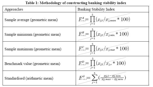where x_j,t is the observed value of a CAMEL indicator j for the period ‘t’ and its sample period average, minimum, maximum and benchmark values are x_j,mean, x_j,min, x_j,max, and x_j,o, respectively. For construction of the Index F^D, we set the benchmark value of x_j,o, based on sample statistics and applied perspectives. Accordingly, we used benchmark value for capital adequacy ratio at 10 per cent in line with the regulatory requirement and the sample minimum values for other indicators i.e., NPA ratio at 2 per cent, operating expenses and provisions ratio at 3 per cent, return on assets at 0.9 per cent, and liquidity ratio 30 per cent. Furthermore, it is to be noted that empirical CAMEL indicators can have differential implications for financial stability. Illustratively, higher CRAR could imply for risk aversion and lower leverage and thus, improvement in financial stability. Similarly, higher return on asset and liquidity ratio could be positively associated with financial stability. However, an increase in the proportion of non-performing loans in total loans could imply for deterioration of asset quality and financial instability. Similarly, higher operating cost ratio could imply for managerial inefficiency and financial instability. Therefore, we used inverse of NPA and operating expense indicators for constructing their indices, so that all CAMEL indicators could be linked with financial stability in the same direction.

As regards data, we collected information from various sources including the RBI, CMIE, NSE and individual bank websites. We had to engage in data mining to create consistent series of CAMEL indicators for a reasonably longer period. Illustratively, we could obtain data for deriving CAMEL indicators for 39 banks comprising most public sector banks and some of the old and new private sector banks for the period 1997:Q1 to 2012:Q3. We extended the series to begin from 1995:Q2 by using annual balance sheet data and extrapolation method*. It may be mentioned that these 39 banks accounted for more than three-fourth share of total banking sector (Table 2).

* For extrapolation purpose, we used TRAMO-SEATS available in Eviews software.

Section IV
Indian Banking System: Some Stylised Facts

India adopted reform in the early 1990s in the wake of balance of payment crisis. The reform began with a focus on financial sector in general and the banking system in particular, as the latter constituted the principal component of financial system. As part of reform, the banking sector was granted greater freedom in deposit mobilisation, allocation of credit and pricing decisions. Competition in the banking system was promoted by allowing new private sector banks and greater access of foreign banks. The regulation and supervision system embraced prudential regulation based on international standards such as Basel principles. In order to support the banking sector operate effectively and efficiently, financial markets were developed through newer instruments and modern technology. Monetary policy framework shifted focus from direct instruments such as reserve requirement to indirect instrument such as interest rate and liquidity adjustment facility.

The reform led banking system showed significant improvement in terms of soundness, operational and allocation efficiency parameters (Table 3). Illustratively, during 1995-96, the capital adequacy ratio (CRAR) for the entire banking system stood at 8.7 per cent with 75 banks showing capital adequacy ratio (CRAR) above the regulatory requirement of 8 per cent and 17 banks showing CRAR below 8 per cent. In the wake of the Asian crisis, the regulatory capital adequacy requirement was increased to 9 per cent by March 1998. Since then banks have shown sustained improvement in meeting the capital requirement above the stipulated minimum. During 2007-08, the CRAR for the banking system stood at 13 per cent, 400 basis points higher than the minimum regulatory requirement. Similarly, asset quality showed steady improvement as the ratio of gross non-performing loans to gross advances ratio declined from as high as 17 per cent in 1995-96 to 2.4 per cent during 2007-08. Managerial efficiency improved with operating expenses to total assets ratio declining by one percentage point between 1995-96 and 2007-08. The liquidity ratio showed a moderation of 10 percentage points reflecting the impact of SLR reduction to enable banks for providing increased credit to private sector to support growth, which is reflected in rising trend in credit-deposit ratio (CDR). The profitability indicator, which showed a volatile trend during the 1990s, exhibited stability as the return on asset ratio hovered around 1 per cent during 2002-03 to 2007-08. After the global crisis, bank indicators have shown some weaknesses especially during the last two years. There has been moderation in capital adequacy indicator, increase in NPA ratio, and rising operating expenses reflecting upon the impact of macroeconomic conditions.

Section V
Empirical findings

As common to time series analysis, our empirical analysis begins with unit root test of economic and financial variables including output, prices, interest rate and banking sector’s CAMEL indicators and the financial stability index as shown in Table 4. We find that during the sample period, the output indicator, real GDP (excluding agriculture and public administration) in levels after seasonal adjustment and log transformation, turned out to be non-stationary but stationary process in terms of first difference and year-on-year growth. Similarly, the wholesale price index turned non-stationary in level form but stationary in first difference form. The call money interest rate can be stationary in level form. Among banking indicators, three of the CAMEL indicators pertaining to capital adequacy, asset quality and managerial efficiency were found to be non-stationary variables in levels but stationary processes in their first differences. On the other hand, return on assets and liquidity ratio indicators could be stationary in levels. Thus, the index of financial stability, after seasonal adjustment and log transformation, turned out to be non-stationary in level but stationary in first difference.

Deriving from the unit root analysis, we estimated VAR models comprising alternative combinations of stationary variables in first differences. Following the arguments of Dhal (2012), we also include in the VAR models two exogenous variables pertaining to oil price shock (first difference of log transformed mineral oil price index) and food price inflation (first difference of seasonally adjusted and log transformed food price index) in order to account for the supply shocks. Table 5 provides summary statistics of these VAR models. Alluding to our discussion earlier, the VAR models with banking stability index based on various sample statistics show similar system properties. Thus, we considered two alternative indicators of stability: the calibrated index (F^D), geometric mean index and the standardised index (F^S), arithmetic mean index. The summary statistics of the VAR models validate the model with financial stability as compared with the model without this indicator. Illustratively, consider the two VAR models; VAR1 comprising three variables, namely, the first differences of seasonally adjusted and log transformed real GDP (dY) and Price Index (dP) and call money rate (r) and VAR 2 which additionally included the first difference of seasonally adjusted and log transformed financial stability indicator (dF). The model with financial stability indicator (VAR2), as compared with the model without financial stability (VAR1), could be validated in terms of predictive power as reflected in higher value of log-likelyhood, lower value of the determinant of residual covariance matrix and better i.e. lower value of information criteria. Thus, for further analysis we confine our discussion to VAR models based on banking stability index, F^D and ^FS.

Taking the analysis further, Table 6 provides results for Granger non-causality block exogeneity test for two VAR models with financial stability indicator. Results show that financial stability can share statistically significant bi-directional Granger causal relationship with macroeconomic variables including output, price and interest rate taken together. Thus, financial stability can be considered as an endogenous variable in the VAR model. As regards other variables, output and interest rate shared significant bi-directional Granger causal relationship with other variables. The price variable Granger caused other variables. It was also Granger caused by other variables, albeit, at higher level of significance at 10 per cent.

V.1 Impulse response analysis

In a VAR model, impulse responses can vary according to the order of the variables appearing in the model. Thus, we considered two types of impulse responses: Choleski decomposition procedure and generalised impulse responses owing to Peasaran and Shin (1997). Interestingly, both types of impulse responses appeared to be more or less similar. Thus, we focus on the Choleski impulse responses of the VAR model with output, price, interest rate and financial stability indicator appearing in that order. Since our objective is to assess total impact of a variable on other variables over shorter and medium-longer horizons, we considered accumulated responses. The impulse responses of variables along with asymptotic standard error bands arising from the VAR model with financial stability indicator are shown in Annex 1 and 2. The impulse response analysis provides answers to some of the critical issues we raised in the beginning. In this regard, we cull out the impulse responses (suppressing the associated standard error) as provided in the Annex for the following discussion.

V.1.1 Impact of financial stability on the macro indicators

We first consider the impact of financial stability on macro indicators, viz., output growth, inflation and interest rates. From the model estimated with first differences of output (dY), prices (dP), financial stability (dF) and interest rate (r) in level, we found that a positive one standard deviation shock to financial stability could be associated with positive responses of both output and price variables accompanied by softer interest rate (Chart 1). It was evident that financial stability could have significant impact on growth over the medium term between 8 to 24 quarters as the impact beyond 24 quarters could not be statistically significant due to large standard errors. Moreover, financial stability impact on output growth at about 1.2 per cent at 24-quarters horizon was substantially higher than the inflation impact at 0.25 per cent. This implies that financial stability could promote economic growth without much threat to price stability over medium-longer horizon.

V.1.2 Impact of macroeconomic conditions on financial stability

Second, a positive standard deviation shock to output growth, implying greater economic stability could be associated with enhanced financial stability (see Table 7). However, a positive standard deviation shock to the inflation rate implying price instability could adversely affect financial stability. In absolute terms, both inflation and growth shocks had more or less similar impact on financial stability over the medium to long term horizon. Thus, economic stability and price stability could promote financial stability.

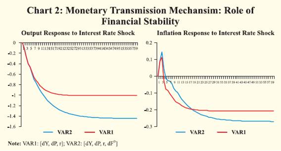
V.1.3 Effectiveness of monetary transmission: Role of financial stability

Thirdly, a positive standard deviation shock to interest rate, reflecting upon tight monetary policy stance, can contain inflation but adversely affect growth and financial stability. However, in terms of size, its impact on financial stability could be much lower than growth and inflation effects. A comparative picture of the output and inflation responses to call money rate shock arising from the model without financial stability (VAR1) and the model with financial stability (VAR2) provides insights about the role of financial stability in influencing the effectiveness of monetary policy (see Chart 2). In this case, we find that financial stability does not affect effectiveness of monetary transmission mechanism in the shorter horizon. However, in medium and longer horizons, output and inflation responses to monetary policy stance could be a sizably enhanced due to financial stability. This is evident from output and inflation responses to the call money rate shock arising from the model with financial stability being 30 to 40 per cent higher than the model without financial stability. Thus, financial stability can contribute to medium-longer term effectiveness of monetary policy in macroeconomic stabilisation.

V.1.4 Persistence of Growth and Inflation: Role of Financial Stability

Fourthly, a comparison between the two VAR models with and without financial stability indicator also shows the changes in the nature of output and inflation persistence to their own shocks (see Chart 3). With the presence of financial stability indicator, output shock could be more persistent and inflation less persistent over medium and longer horizon. From a comparative perspective between output and inflation, the increase in persistence of output is much higher than the moderation of persistence in inflation owing to financial stability. Following Cochrane (1988) and Campbell and Mankiew (1987), persistence in economic time series can reflect on the importance of their permanent component relative to transitory component. Accordingly, the role of financial stability in influencing output and inflation persistence can be interpreted.

V.1.5 Interest rate’s response to growth and inflation: Role of financial stability

The impulse response analysis provides insights about how interest rate would react to growth and inflation shocks with and without the presence of financial stability in the VAR model (see Chart 4).

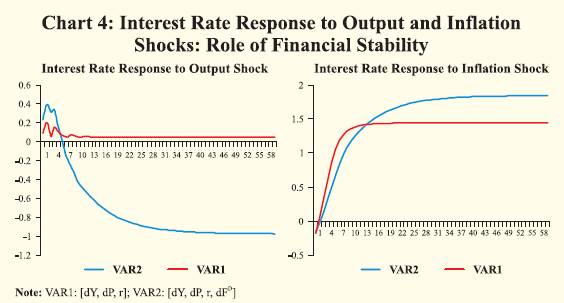Illustratively, in the model without financial stability (VAR1), interest rate reacts positively to positive shocks to both output and inflation indicators, though the interest rate’s response to price shocks is substantially higher than its response to output shock. This finding could be attributed to greater sensitiveness of policy rate to price stability than economic growth. However, in the presence of financial stability, i.e., VAR2 model, interest rate continues to react positively to inflation shock and such reaction is enhanced in the medium term. On the other hand, in response to output shock, interest rate reacts positively, albeit marginally, in the short run but negatively and substantially in the medium-longer horizon as compared with its short run response. This implies that financial stability could facilitate softer policy to promote growth and tighter policy to achieve price stability in the mediumlonger horizon.

Section VI
Conclusion

In this study, we endeavoured at providing applied perspectives on some crucial policy issues relating to the relationship of financial stability with growth and inflation which characterise economic stability and monetary stability objectives. We experimented with aggregate banking sector soundness index comprising prudential CAMEL indicators based on quarterly data for a sample of 39 banks comprising all public sector banks and major old and new private sector banks. We used an augmented VAR model for analysing the transmission mechanism. Our empirical investigation brought to the fore some interesting perspectives. First, financial stability, growth and inflation could share a medium to longer term relationship, and this finding is in line with several studies. Second, financial stability can promote growth without posing much threat to price stability. Third, financial stability can enhance the effectiveness of monetary transmission mechanism. Fourth, economic growth can have positive influence on financial stability. But inflation can adversely affect financial stability. Finally, with financial stability, growth could be more persistent and inflation less persistent. Since persistence could imply for permanent component, we can infer that financial stability will be beneficial for growth and price stability. Thus, we conclude that financial stability goal can be pursued along with conventional objectives in the Indian context.

These findings are expected to be useful for policy purposes. Going forward, research on the subject could be extended inter alia through two major directions. First, attempts can be made towards constructing a quarterly index of financial stability index comprising CAMEL indicators and financial market indicators for reasonably longer period to examine further perspectives on the subject. Second, on the methodological front, VAR models with Bayesian analysis and sign restrictions on impulse response and structural identification could be useful. In addition, attempts can be made to use the VECM to explore long-run relationship between financial stability and macroeconomic indicators.

References

Ang, J. B. 2008. “What are the mechanisms linking financial development and economic growth in Malaysia?” Economic Modelling, 25: 38-53.

Azariadas, C., Smith, B. 1996. “Private Information, Money and Growth: Indeterminacies, Fluctuations, and the Mundell-Tobin effect.” Journal of Economic Growth, 1: 309-322.

Bagehot, W. 1873. Lombard Street: A Description of the Money market. Irwin, Homewood, Ilinois.

Bank for International Settlement. 2010. “Assessing the macroeconomic impact of transition to stronger capital and liquidity requirement.” Final Report, BASEL.

Bernanke, B. S., Kuttner, K. N. 2005. “What Explains the Stock Market’s Reaction to Federal Reserve Policy?” Journal of Finance, 60(3):1221-1257.

Bordo, M. D., Murshid, A. P. 2000. “Are Financial Crises Becoming Increasingly More Contagious? What is the Historical Evidence on Contagion?” NBER Working Papers 7900.

Borio, C. 2003. “Towards a macroprudential framework for financial supervision and regulation?” CESifo Economic Studies, 49:181-216.

Borio, C., English, B., Filardo, A. 2003. “A tale of two perspectives: old or new challenges for monetary policy?” BIS Working Papers 127.

Borio, C., Lowe, P. 2002. “Asset prices, financial and monetary stability: exploring the nexus.” BIS Working Papers 114.

Borio, Claudio. 2006. “Monetary and financial stability: Here to stay?” Journal of Banking & Finance, 30:3407-3414.

Boyd, J. H., Smith, B. D. 1998. “Capital market imperfections in a monetary growth model”, Economic Theory, 11, 241-273.

Boyd, J. H., Levine, R., Smith, B. D. 2001. “The impact of inflation on “financial sector performance.” Journal of Monetary Economics, 47:221-248.

Braun, P. A., Mittnik, S. 1993. “Mis-specifications in Vector Autoregressions and Their Effects on Impulse Responses and Variance Decompositions.” Journal of Econometrics, 59:319-341.

Calderon, C., Duncan, R., Schmidt-Hebbel, K. 2004. “The role of credibility in the cyclical properties of macroeconomic policies: Evidence for emerging markets.” Review of World Economics, 140(4):613-633.

Calvo, G. 1997. “Capital flows and macroeconomic management: Tequila lesson.” International Journal of Finance and Economics, 1(3):207-223.

Campbell, John Y., and N. Gregory Mankiw. 1987. “Permanent and transitory components in macroeconomic fluctuations.” American Economic Review, 77(2): 111-117.

Cevik, E. I., Dibooglu, S., Kenc, T. 2013. “Measuring financial stress in Turkey”, Journal of Policy Modeling, 35: 370-383.

Choi, S., Boyd, J., Smith, B. 1996. “Inflation, financial markets, and capital formation”, Federal Reserve Bank of St. Louis Review, 78: 9-35.

Cochrane, John H. 1988. “How Big is the Random Walk in GNP?”, Journal of Political Economy, 96(5):893-920.

Cook, T., Hahn, T. 1989. “Federal Reserve Information and the Behaviour of Interest Rates”, Journal of Monetary Economics, 24:331- 351.

Cukierman. 1992. Central Bank Strategy, Credibility and Independence: Theory and Evidence. Cambridge, Mass, MIT press.

Demetriades, P. and Hussein, K. 1996. “Does Financial Development Cause Economic Growth?: Evidence for 16 Countries”, Journal of Development Economics, 51:387-411.

Demirguc-Kunt, A., Levine, R. 1996. “Stock Market Development and Financial Intermediaries: Stylized Facts”, World Bank Economic Review, World Bank Group, 10(2):291-321.

Diamond, D. W., and R. G. Rajan. 2006. “Money in a Theory of Banking.” American Economic Review, 96 (1): 30–53.

———. 2012. “Illiquid Banks, Financial Stability, and Interest Rate Policy.” Journal of Political Economy,120 (3): 552–91.

Dovern, J., Meier, C., Vilsmeier, J. 2010. “How resilient is the German banking system to macroeconomic shocks?” Journal of Banking & Finance, 34:1839-1848.

Driffill, J., Rotondi, Z., Savona, P., Zazzara, C. (2006): “Monetary policy and financial stability: what role for the futures market?”, Journal Financial Stability, 2, 95–112.

Eichberger, J., Summer, M. 2005. “Bank Capital, Liquidity, and Systemic Risk”, Journal of the European Economic Association, 3(2):547-555.

Eichengreen, B., Arteta, C. 2000. “Banking Crises in Emerging Markets: Presumptions and Evidence”, Center for International and Development Economics Research Working Paper No. 115.

Gambacorta, L.2011. “Do Bank Capital and Liquidity Affect Real Economic Activity in the Long Run? A VECM Analysis for the US”, Economic Notes, 40(3):75-91.

Ghosh, S. 2011. “A Simple Index of Banking Fragility: application to Indian Data”, Journal of Risk Finance, 12(2):112-120.

Goodfriend, M. 1987. “Interest rate smoothing and price level trendstationarity”, Journal of Monetary Economics” 19:335-348.

Graeve, F. De, Kick, T., Koetter, M. 2008. “Monetary policy and financial (in)stability: An integrated micro–macro approach”, Journal of Financial Stability, 4(3):205-231.

Granville, B., Mallick, S. 2009. “Monetary and financial stability in the euro area: Pro-cyclicality versus trade-off”, Journal of International Financial Markets, Institutions and Money, 19(4):662-674.

Herrero, A. G., Rio, P. 2003. “Financial Stability and the Design of Monetary Policy”, Banco de Espana Working Paper No. 0315.

Huybens, E., Smith, B. 1998. “Financial market frictions, monetary policy, and capital accumulation in a small open economy”, Journal of Economic Theory, 81:353-400.

Huybens, E., Smith, B. 1999. “Inflation, financial markets, and longrun real activity”, Journal of Monetary Economics, 43:283-315.

Institute for International Finance (IIF). 2011. “The Cumulative Impact on the Global Economy of Changes in the Financial regulatory Framework”, Final Report, September.

Issing, O. 2003. “Monetary and Financial Stability: Is there a Tradeoff?”, BIS Working Paper No. 18.

Kashyap, A.K., Stein, J.C. 1995. “The impact of monetary policy on bank balance sheets”, Carnegie-Rochester Conference Series on Public Policy, 42:151-195.

Kashyap, A.K., Stein, J.C. 2000. “What do a million observations on banks say about the transmission of monetary policy?”, American Economic Review, 90 (3):407–428.

Kindleberger, C.P. 1978. Manias, Panics and Crashes. Basic Books, New York.

King, R., Levine, R. 1993. “Finance and growth: Schumpeter might be right”, Quarterly Journal of Economics, 108:717-737.

Kishan, R.P., Opiela, T.P. 2000. “Bank Size, bank capital, and the bank lending channel”, Journal of Money ,Credit and Banking. 32(1):121- 141.

Kuttner, K. N. 2001. “Monetary policy surprises and interest rates: Evidence from the Fed funds futures market”, Journal of Monetary Economics, 47(3):523-544.

Liu, W., Hsu, C. 2006. “Role of financial development in economic growth: experiences of Taiwan, Korea, and Japan”, Journal of Asian Economics, 17:667-690.

Locarno, A. 2011. “The macroeconomic impact of Basel III on the Italian economy”, Occasional Papers No. 88, Banca D’ Italia.

McKinnon, R. 1973. “Money and Capital in Economic Development”, Brookings Institution, Washington DC.

Minsky, H. 1991. The Financial Instability Hypothesis: A Clarification. in: M. Feldstein, ed., The Risk of Economic Crisis, University of Chicago Press: Chicago, 158-70.

Mishkin, F. S. 1996. “The Channels of Monetary Transmission: Lessons for Monetary Policy”, NBER Working Paper No. 5464.

Odedokun, M.O. 1996. “Alternative Econometric Approaches for Analyzing the Role of the Financial Sector in Economic Growth: Time Series Evidence from LDCs”, Journal of Development Economics, 50(1):119-146.

Padoa-Schioppa, T. 2002. “Central Banks and Financial Stability: Exploring a Land in Between”, 2nd ECB Central Banking Conference.

Patrick, H. 1966. “Financial Development and Economic Growth in Underdeveloped Countries”, Economic Development and Cultural Change. 14(2):174-189.

Poloz, S. S. 2006. “Financial stability: A worthy goal, but how feasible?”, Journal of Banking & Finance, 30: 3423-3427.

Rajan, R. G. 2005. “Has Financial Development Made the World Riskier?” NBER Working Paper No. 11728.

Robinson, J. 1952. The Generalisation of The General Theory in: The Rate of Interest and other Essays. McMillian, London.

Rotondi, Z. and Giacomo V. 2005. “The Fed’s reaction to asset prices”, Journal of Macroeconomics, 30: 428-443.

Rousseau, P. L., Wachtel, P. 2002. “Inflation thresholds and the finance– growth nexus”, Journal of International Money and Finance, 21:777- 793.

Rousseau, P. L., Yilmazkuday, H. 2009. “Inflation, financial development, and growth: A trilateral analysis”, Economic Systems, 33:310-324.

Rudebusch, G. D. 2005. “Monetary Policy Inertia: Fact or Fiction?”, International Journal of Central Banking, 2(4):85-135.

Schumpeter, J.A. 1911. The Theory of Economic Development. Oxford University Press, Oxford.

Schwartz, A. J. 1995. “Why Financial Stability Depends on Price Stability”, Economic Affairs, 21-25.

Shaw, E. 1973. Financial deepening in economic development. Oxford University Press, New York.

Sims, C. A. 1992. “Interpreting the macroeconomic time series facts: The effects of monetary policy”, European Economic Review, 36:974- 1011.

Sinha, A., Kumar, R., and Dhal, S.C. 2011. “Financial Sector Regulation and Implications for Growth”, CAFRAL-BIS International Conference on Financial Sector Regulation for Growth, Equity and Financial Stability in the post-crisis world.” BIS Paper No. 62.

Slovik, P. and B. Cournède. 2011. “Macroeconomic Impact of Basel III”, OECD Economics Department Working Papers No. 844, OECD.

Smith, R.T., Egteren, V. H. 2004. “Interest Rate Smoothing and Financial Stability”, Working paper, University of Alberta, Edmonton, Canada.

Subbarao, D. 2011. “Price stability, financial stability and sovereign debt sustainability policy challenges from the New Trilemma”, Second International Research Conference of the Reserve Bank of India, Mumbai, February 2012.

Subbarao, D. 2009. “Financial stability - issues and challenges”, FICCI-IBA Annual Conference on “Global Banking: Paradigm Shift”, organised jointly by FICCI and IBA, Mumbai, 10 September 2009.