Rajib Das and Siddhartha Nath*

This paper assesses the adequacy of foreign exchange reserves in India following several instances of stress in the external sector. It is observed that India’s foreign exchange reserves are higher than those of many countries with similar external sector characteristics like current account deficits and high foreign portfolio investment inflows, and also in relation to several ‘rules of the thumb’ for reserve adequacy. Empirical analysis suggests that India’s reserve holdings are adequate and largely explained by several precautionary motives of reserves’ accumulation in light of its growing external sector openness and the associated risks. A calibration of an optimization model by Jeanne and Ranciere (2011) for India also suggests that India’s foreign exchange reserves are adequate to cover potential stress scenarios.

JEL Classification : E58, F31, F32, F37 and F41.

Keywords : Foreign Exchange Reserves, External Sector Vulnerability, Precautionary Demand for Reserves, Capital Flows, Current Account, Crisis.

Introduction

India’s external sector has been extensively liberalized during the last two decades and the share of the external sector in GDP has increased steadily. The share of merchandise exports and imports in GDP increased from 11 and 15 per cent on average during 2000/01-2007/08 to 15 and 24 per cent respectively during 2008/09-2014/15. Inflows of foreign portfolio investments (equity and debt combined) increased from 0.9 per cent to 1.6 per cent of GDP over the same time periods.¹

The country’s enhanced global exposure, however, has made it more vulnerable to volatilities in international trade, commodity prices and cross-border financial flows. India experienced some form of international contagion following several financial crises like the Mexican crisis in 1994-95, the East Asian crisis in 1997-98, the sub-prime financial turmoil in 2008-09, the Euro debt crisis in 2010-11 and the Fed’s ‘taper tantrum’ in 2013-14.² Such turmoil was followed by a number of interventions by the Government of India and the Reserve of Bank of India (RBI) -- market-based (for example, spot and forward sales of foreign exchange (US$), tightening of domestic interest rates) and administered (for example, restrictions imposed on flexibilities of importers and exporters, stricter prudential norms on currency trade, curtailed freedom on the derivatives position like cancelation and rebooking of forward contracts or trading in currency futures and options), which aimed to minimize the impact of these crises on the country’s financial sector.³ Such interventions also include those by RBI in the form of buying and selling of foreign exchange that can influence reserves. Foreign exchange interventions by RBI can, however, also take place during normal times with the motive of smoothening excessive currency fluctuations and building reserves for ‘precautionary’ motives.

In this paper, foreign exchange reserves include foreign currency assets, reserve tranche positions and special drawing rights (SDRs) of the International Monetary Fund (IMF). India’s stock of reserves increased from US$ 145.9 billion in 2005-06 to US$ 322.6 billion in 2014-15. This build-up of reserves can be explained primarily by an increase in foreign capital inflows, which are the main source of financing high and persistent current account deficits (CAD). For example, the annual average CAD was 3 per cent of GDP between 2008 and 2014.

Holding foreign exchange reserves entails both benefits and costs. Reserves can provide liquidity buffers, smoothen external shocks and potentially avoid disruptive output adjustments. Emerging markets with adequate reserve holdings ahead of the global financial crisis in general suffered smaller output and consumption declines (IMF 2013). However, carrying reserves also entails costs such as the interest sacrificed on reserve holdings. Therefore, assessing whether reserves are adequate and at what level, remains an important question for most countries.

This paper assesses reserve adequacy in India during 1996-2014 using three distinct approaches: (i) peer comparison, (ii) an econometric estimation of a reserve demand function, and (iii) simulation of a rational optimization model of reserve holdings under different crisis scenarios.⁴ The paper finds that India’s stock of reserves was much higher than the level maintained by countries with similar external sector characteristics. Econometric estimations and simulations of the optimization model also suggest that India’s reserves are adequate to cover a broad set of external sector risks.

A large body of literature examines the issue of reserve adequacy and discusses several motives for reserve holdings.⁵ Literature emphasizes both the short-term and the longer-term motives of holding reserves. The longer-term factors include precautionary and insurance motives against unforeseen external shocks, as well as the mercantilist gains to be reaped by keeping the domestic currency undervalued. Aizenman and Marion (2002), Edison (2003), Gosselin and Parent (2005), Park and Estrada (2009) and IMF (2011) estimate reserve demand equations emphasizing the precautionary motive, while Ghosh et al. (2012) document the mercantilist motive for emerging market economies. Short-term factors include, for example, monetary disequilibrium characterized by excess money supply or demand over and above what can be explained by standard determinants such as real GDP, nominal interest rate and exchange rate. Other short-term motives for holding reserves include buffers against external payment gaps and their potential use to counter volatility in cross-border capital flows.

The short-term factors affecting reserve holdings are best categorized as inventory adjustments towards a desired level determined by the two long-run factors (Prabheesh et al., 2009). However, this necessitates a prior approach on desired reserve levels, which is the subject of investigation in this paper. Therefore, the empirical framework adopted in this paper broadly captures long run motives.

Among the limited studies in the Indian context, Sehgal and Sharma (2008) and Mishra and Sharma (2011) analyse the short-run dynamics of reserve accumulation in India with particular focus on monetary disequilibrium. Ramachandran (2004), on the other hand, derives the optimum reserves for India using external payment imbalances and the opportunity costs of holding reserves as the benchmark variables. The empirical exercises in these studies also find that India’s reserves are broadly adequate to cover the risks on both domestic and external fronts. However, existing studies are mostly restricted to short-run reasons for the accumulation of reserves. In contrast, the focus of this paper is on longer-term motives.

The rest of the paper is organized as follows: Section II presents some stylized facts on India’s reserves. This section also revisits some of the conventional thumb rules for reserve adequacy. Section III describes the three methodologies used for assessing India’s reserve adequacy and analyses the findings followed by conclusions in Section IV.

Section II

India’s Foreign Exchange Reserves: Stylized Facts

India’s foreign exchange reserves have grown substantially since 2000 and stood at US$ 334 billion as of end-August, 2015, as compared to US$ 107.4 billion at end-March, 2004. In fact, the reserves reached US$ 300 billion by the end of 2007-08, and have fluctuated around this level since then (Chart 1).

Although the accumulation of reserves has gained some pace since the middle of 2013-14, reserves in relation to GDP declined since the global financial crisis - from 94 per cent in Q1 2008-09 to 60 per cent in Q3 2013-14. Besides revaluation, the increase in reserves, from the early 2000s till the global financial crisis, was primarily on account of the increase in foreign portfolio investment (FPI) inflows (Chart 2).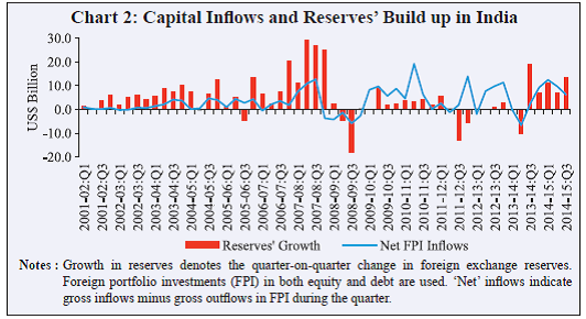

India’s CAD was relatively low during this period (on average about 0.1 per cent of GDP between 2001 and 2007), and therefore increasing capital inflows were associated with the accumulation of reserves. India’s reserves increased by US$ 232 billion between Q1 2001-02 and Q1 2008-09, a period of cumulative net FPI inflows of US$ 66.3 billion. On the other hand, while there were cumulative net FPI inflows of US$ 137 billion between Q4 2008-09 and Q3 2014-15, a large part of these inflows could not be accumulated as reserves due to large CAD. In fact, reserves increased only by US$ 65 billion during these years owing to a high CAD, which on average was 3 per cent of GDP. As the current account deficit moderated during 2014-15, India’s reserves accumulated further.

Are the current levels of reserves adequate for India in terms of standard indicators? From an international trade perspective reserves equivalent to three months of import coverage are conventionally used as a thumb rule for their adequacy for most of the developing countries. With increasing global financial integration, alternative thumb rule measures of reserve adequacy such as reserves equivalent to 20 per cent of the broad money and 100 per cent coverage of outstanding short-term external debt with residual maturity of 1-year (the Greenspan-Guidotti rule) are increasingly being adopted in several countries.

These adequacy benchmarks against imports and short-term external debt broadly capture the notion of reserves providing a cushion against external payment imbalances. The thumb rule against 20 per cent of broad money on the other hand captures the risks of capital flight, or massive outflows of deposits encountered during a crisis.⁶

Reserves in India have remained fairly above the adequate level in terms of 3-months of import coverage (Chart 3) and also above the country’s outstanding short-term external debt with residual maturity (Chart 4) since 2004/05. However, they have fallen below the threshold of 20 per cent of broad money (Chart 5) since 2010-11.

Notes : Charts 4 and 5 compare India’s foreign exchange reserves against short-term external debt and 20 per cent broad money, respectively. Short-term external debt is measured at residual maturity of at most a year.

Although operationally useful, these indicators largely focus on a single aspect of risk in assessing reserve adequacy. Moreover, the threshold limits are somewhat arbitrary. Also, different indicators may provide conflicting pictures on reserve adequacy. An alternative methodology is considering benchmarks based on cross-country experiences. For instance, IMF (2011) assesses the potential sources of resource drainage in emerging market economies (EMEs) based on the experiences of a number of countries. It has developed a risk-weighted metric of reserve adequacy covering several potential sources of resource drainage during events of exchange market pressures. Based on this approach, reserve holdings in the range of 100-150 per cent of the metric or above are considered adequate. The metric proposed for EMEs is:

IMF Metric = (0.3 * STED + 0.1 * OPL + 0.05 * M₃ + 0.05 * X)

where STED indicates the short-term external debt with residual maturity of one year. OPL indicates the ‘other portfolio liabilities’ which include equity securities held with foreigners, outstanding short-term trade credits and any other short-term liability to the government, central bank, commercial banks and corporates. The variables M₃ and X denote broad money and exports, respectively. Reserves in India amount to 193 per cent of the IMF metric (Chart 6), and based on the 100-150 per cent threshold, are ‘adequate’ to cover a broad set of external sector risks.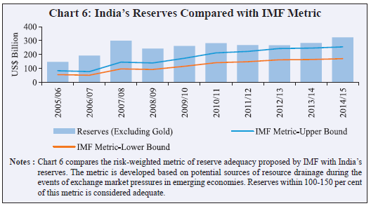

The indicators of reserve adequacy discussed here are simple. However, the thresholds may not always be pertinent for different countries which largely differ in their external exposures in both trade and capital accounts. Also, the channels of vulnerability to external crises differ across countries. Importantly, the thresholds may not remain relevant across different time periods even for a particular country. India has witnessed increasing global integration over the past two decades. Several crises since 2008 and the policies followed globally also increased the chances of external imbalances and large capital outflows. This may require the reserve adequacy thresholds to be re-examined and redefined over time. Therefore, this paper systematically assesses India’s reserve adequacy by taking into account several macroeconomic risk factors – both country specific and global - over the last two decades.

Section III

Empirical Analysis

The paper used three distinct approaches for assessing the reserve adequacy in India: (i) comparisons with appropriate peers, (ii) econometric estimation of a reserve demand function, and (iii) simulation of a rational optimization model of reserve holdings under different crisis scenarios (all data definitions and sources used to implement the methodologies are described in Annexure I). The three methodologies are now discussed in detail.

III.1. Peer Comparison of Reserve Holdings

Methodology

India’s reserve holdings were compared with a set of countries with similar external sector characteristics. The comparator countries include developing economies like Brazil, Chile, Colombia, Czech Republic, Egypt, Mexico, Pakistan, Poland, Romania, South Africa and Turkey and also advanced economies like Australia, Canada, Greece, Italy, Portugal, Spain, United Kingdom and USA. The countries selected for this exercise were among the top 50 economies measured by the average nominal GDP (US$) during 2008-14 and are also those, which on average like India, had current account deficits of more than 1 per cent of GDP during this period. Reserve holdings (excluding gold) are expressed as percentage of the (i) size of the economy, that is, nominal GDP, and (ii) imports. The reserve position for these countries is compared for two time periods, 2008-14 and 2001-07. Although the sources of reserve accumulation varied across these countries, the average FPI equity inflows (as percentage of GDP) are shown as a proxy for volatile capital account activities for these countries.⁷ Reserve holdings together with FPI equity inflows (as percentage of GDP) are expected to show the underlying risks to the external sector of a country that is emerging from private capital flows.

Findings

India’s reserves remained higher (in relation to both GDP and imports) in general than most of the developing countries (Table 1). However, in recent years FPI inflows in relation to GDP were much higher in India than those in most developing countries. On the contrary, the current account deficit in India was much lower. Advanced economies generally held lesser reserves, as they, barring Australia, held dollar liquidity swap lines.

While reserves as a share of GDP increased during 2008-14 (as compared to 2001-07) from 15.9 per cent to 16.4 per cent, they declined as a share of imports from 85 per cent to 58 per cent over the same period in India. The increase in reserves as a share of GDP in the recent period was partly due to high FPI inflows which masked the increasing current account deficit. Although equity flows remained roughly at the same level between the two periods, FPI debt inflows to India have increased remarkably since 2011 as ceilings on debt investments were raised within a short span of time. The reserves to imports ratio deteriorated after the global financial crisis as imports increased and the current account deficit widened. Imports increased at an annual rate of 12.8 per cent while reserves grew by 7.1 per cent annually between 2006 and 2013.

III. 2. Econometric Estimation of Reserves’ Demand Function

Methodology

While a comparison with appropriate peers is useful, an assessment of reserve adequacy needs a more systematic examination vis-à-vis a set of potential sources of external vulnerability. External sector stress could emanate from uncertainties in both the current account and capital flows, which have increased over time in India, and may have a significant influence on the demand for reserves. The average current account deficit was 4.5 per cent of GDP during 2011 and 2012, which was much higher than the average of 1.0 per cent for 2004-07. Volatility in capital inflows, measured by the standard deviation of the monthly FPI inflows in debt and equity combined, also increased sharply from US$ 1.0 billion in 2006 to US$ 4 billion in 2013; they, however, moderated to US$ 2 billion in 2014. India also witnessed events of large capital outflows during external shocks such as the collapse of Lehman Brothers, and the Fed’s ‘taper tantrum’. The econometric exercise described in this section estimates the reserves’ demand by taking into account several such factors.

The key variable for capturing reserves’ demand in the econometric model is the reserves to GDP ratio. The explanatory variables can be broadly classified into three major categories: (i) external sector health and risks to both the current and capital accounts measured by variables such as imports to GDP ratio, nominal effective exchange rate (NEER), volatility of current account receipts, volatility of foreign capital inflows measured by the volatility in FPI inflows and broad money to GDP ratio, (ii) possible motives of ‘mercantilism’ indicated by the undervaluation of the trade weighted real effective exchange rate (REER) (where undervaluation is measured by the deviation from the Hodrick-Prescott filtered trend), and (iii) the opportunity cost of holding reserves measured by the interest rate differential between India and the United States (difference between yields in 91-day treasury bills). It is hard to distinguish between the precautionary and insurance motives empirically. Broadly therefore, the variables representing external sector risks account for these motives jointly.

The estimating equation is specified as:

The estimating equation is broadly in line with the specifications used in literature. The imports to GDP ratio is a proxy for current account openness as also a major channel of domestic economic activity, and therefore, is a robust determinant of reserves across various studies. With a higher degree of openness, demand for reserves is expected to increase (i.e. α₁>0).⁸

An appreciating rupee, which is reflected in a higher NEER, makes India’s exports costlier and adversely affects the current account. Also, appreciation in the domestic currency attracts larger foreign capital. Capital flows put the country’s external sector at risk of sudden outflows once NEER starts depreciating. Therefore, an appreciating NEER is likely to increase the demand for reserves (i.e. α₂>0).

Volatility in earnings from exports of goods and services is another factor that can drive the precautionary demand for reserves (Ghosh et. al., 2012; IMF, 2011). This paper, however, uses volatility in current earnings (on both merchandise and invisibles) instead of volatility of only exports (merchandise) as invisibles contribute to a significant portion of the current account in India (averaging almost 45 per cent during 2005-14).

Volatility of FPI inflows is also used as a driver of precautionary reserve demand as it constitutes a significant source of financing of current account deficit in India. In fact, FPI inflows as percentage of GDP in India are significantly higher than many other countries with similar external sector characteristics (Table 1). Moreover, the volatility of capital flows increased over time, especially since 2011 since the debt inflows were liberalized in stages.⁹

Volatility in both current earnings and FPI inflows measured in a quarter is the preceding 24-quarters’ moving coefficient of variation. This measure captures the volatility episodes that may have been built over a fairly long time period. We expect the estimated coefficients on both the volatility of export earnings and capital flows to be positive (that is, α₃ and α₄>0).

The domestic monetary base, measured by the broad money to GDP ratio, is also used as an indicator of the risk of capital flight. Given a variety of capital control measures for residents in India, risks to capital flight will essentially arise from non-residents. The precautionary demand for reserves, therefore, accommodates the higher risk of such capital flight, which could feed into the economy through monetary base (that is, α₅>0).

Finally, the opportunity cost of reserves is the difference between the 91-day treasury bills’ yields in India and the US. The return on the latter, typically, is the proxy of the actual return on reserves while the former is the risk-free return sacrificed by holding reserves in foreign currency. The coefficient of the opportunity cost of reserves is expected to be negative as higher costs of holding reserves should reduce their demand (that is, α₇<0).

Results

Equation (1) has been estimated using OLS on quarterly data covering the period June 1996 (that is, Q1 1996-97) to June 2015 (Q1 2014-15).¹⁰ Table 2 shows the regression results. The estimated coefficients on imports to GDP and volatilities in both the current earnings and FPI inflows are positive and statistically significant. Higher volatility in current earnings and capital flows are both associated with higher reserve demand. The coefficient on NEER and broad money to GDP are also positive and statistically significant. On the contrary, there is not much evidence for the mercantilist motive of reserves’ accumulation as the coefficient on the exchange rate undervaluation is not statistically significant. Further, the coefficient on the opportunity cost of reserves is negative, but not statistically significant, indicating that cost considerations do not play a significant role in explaining the demand for reserves in India. Overall, the results suggest that reserve accumulation in India can be explained by precautionary motives.

Predicted reserves to GDP ratios are obtained by using the estimated coefficients from the empirical model. The square root of the residual sum of squares (RSS) or standard deviation (SD) of the estimated residuals from the model is a measure of the average deviation of the observed reserves to GDP ratio from its predicted value. We use a 2 SD band on predicted reserves/GDP and the 2 SD band are then multiplied by GDP levels for the quarter to calculate the predicted level of reserves. The 2 SD band around the predicted line roughly indicates the interval within which reserves’ demand is likely to persist based on the model with more than 95 per cent confidence.

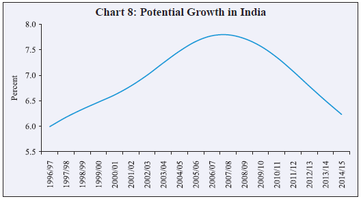
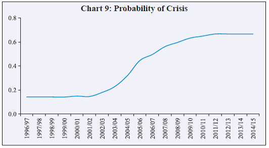
Actual reserves in India remained above the level predicted by the regression for most of the years except for some quarters in 2008-09 and 2009-10, Q1 2011-12 and Q3 2013-14 to Q1 2014-15 (Chart 7). Also, the actual reserves in Q1 2015-16 were higher than the predicted level, indicating that the reserve holdings might have been adequate to cover the broad set of risks as captured in the model. As reserves in India remained within the 2 SD range during the recent period, it may be considered ‘adequate’ under this framework.

III.3. Theoretical Optimization of Reserve Holdings

The regression model provides an understanding of some of the determinants of reserves’ demand and therefore, provides an explanation for the rationale behind holding reserves. However, the underlying assumption is that the authority can take and is always taking an optimal decision on accumulation of reserves and there are ‘no systematic biases towards over-or-under-insurance for the sample as a whole’ (IMF 2011). An alternative approach would be to examine if the actual reserve levels are also consistent with some theoretically optimum reserves obtained against a set of potential risks to the economy. Therefore, this paper calibrated a model of inter-temporal welfare maximization developed by Jeanne and Ranciere (2009, 2011) (henceforth J&R) for an alternate view on optimum reserves in India.

The J&R Model

According to J&R, a risk-averse policymaker aims to maximize the inter-temporal welfare of a representative consumer in a small open economy by smoothening her consumption between pre- and post-crisis periods. It is assumed that the representative consumer loses access to external credit during a crisis. Such a phenomenon is termed ‘sudden stop’, which forces her consumption level to reduce below its long-run path. Therefore, the policymaker enters into an insurance contract with the foreign country in the form of foreign exchange reserves during the normal (that is, no crisis) period, which can be used for meeting contingency requirements and sustaining consumption (through import payments etc.) if the country encounters a sudden stop.

J&R derive the expression for optimum reserves based on a number of parameters to capture external vulnerabilities, domestic growth and the opportunity cost of reserves. The reduced form expression for optimum reserves to GDP (ρ*) ratio is given by:¹¹

An intuitive explanation of the expression suggests that the demand for reserves (in relation to nominal GDP) increases with the probability of a sudden stop (π). Similarly, a higher anticipated loss to the economy owing to a crisis prompts the authority to hold more reserves. Such losses are measured in the model in three ways: First, the extent to which the inflows of external funds reduce during a crisis, or the size of the crisis (λ); second, the possible loss in GDP growth (γ); and finally, the magnitude of real exchange rate depreciation (ΔQ). Reserves’ demand also increases with higher term premium (δ), which is the spread between the longer-term bond return over the short-term, indicating the time preference for investments. Finally, a monetary authority with higher risk aversion (σ) will also demand more reserves than its counterpart with a lower risk aversion. On the flip side, a higher opportunity cost (that is, risk free returns on capital, r) reduces demand for reserves. A country with higher potential growth is also less susceptible to output losses owing to external shocks. Thus, reserves’ demand is also likely to be lower with higher potential growth. p_t is the relative price of a non-crisis dollar in terms of crisis dollar value for global investors which measures the marginal rate of substitution of insurers’ funds in a non-crisis period vis-a-vis that in a crisis period. Finally, x indicates the insurance premium emerging from the sum of Π and δ, and implies that countries with higher crisis probability and lower tolerance for future output losses will be ready to pay higher premium for the insurance or will maintain higher reserves. J&R calibrated these parameters for a sample of 34 middle income countries over 1975-2003 and derived optimum reserves to annual GDP ratio close to 9 per cent.

The J & R Model Parameter Calibration for India

This paper calibrated the model specifically for India by taking some parameters’ values directly from J&R’s paper while estimating the remaining parameters econometrically. The parameters π, λ, γ, g and ΔQ are estimated using the annual data for India during 1996-97 to 2014-15. Term premium (δ), risk free return on reserves (r), and risk-aversion coefficient (σ) are taken from J&R as these parameters are not determined by the country characteristics. δ is the average difference between the 10-year US treasury bill rate and the federal funds rate over 1990-2005 under the assumption that reserves are denominated in US dollars, which is the case for India. r is set equivalent to the short-term dollar interest rate. σ is assumed to be 2, which is the standard value of risk aversion across literature on business cycle and growth.

This paper first defines ‘crisis’ years as years in which either the exports to GDP ratio or the FPI inflows to GDP ratio fell abruptly from the previous year.¹² More precisely, in these years the year-on-year percentage point decline in either of these two ratios was higher than the average fall observed in the sample.¹³ The years 1998-99, 2006-07, 2008-09, 2009-10, 2010-11, 2011-12 and 2013-14 are identified as crisis years. These years broadly capture the known periods of external sector turmoil -- 1998-99 was the year of the East Asian crisis, while the years since 2008-09 broadly cover the global financial crisis, slow recovery in the euro area and slowdown in a number of Asian countries; 2006-07, on the other hand, witnessed relatively high year-on-year decline in FPI inflows responding to a reversal in the monetary policy easing cycle in India.

The probability of crisis (π) was estimated using a probit model, the structure of which is directly adopted from J&R. The dependent variable in the model is a dummy variable indicating crisis episodes (dummy=1 for crisis year). The explanatory variables in the model are real effective exchange rate overvaluations (deviation from its Hodrick-Prescott trend), the central government’s external liability to GDP ratio and financial openness defined as the absolute value of net FPI inflows to GDP ratio. The explanatory variables are taken as the average of their first and second lags. The probit model provides the predicted/estimated probabilities of the crisis. The estimated probability of a crisis varies over time, and allows us to estimate a time-varying optimum reserves to GDP ratio.¹⁴ The study also uses an annual series for the potential growth (g) which is the Hodrick-Prescott trend of the annual growth rate of GDP at factor cost, measured in 2004-05 prices.

Table 3 shows the results of the probit model for estimating crisis probabilities. Higher financial openness is associated with a higher probability of a crisis. On the flip side, the low de facto financial openness reduces the probability of further occurrence of a crisis in the probit model.¹⁵ Real exchange rate overvaluation increases the probability of a crisis but the estimated coefficient is not statistically significant. Estimated potential growth (g) is shown in Chart 8, and the crisis probabilities from the probit model are shown in Chart 9. Potential growth has increased steadily since the mid-1990s, but has declined since 2006-07, which is consistent with several previous studies as well as commentaries by market analysts.¹⁶ The estimated probability has also increased since the early 2000s; it reached its pick in 2010-11 and has remained at that level.

Simulation Scenarios

The parameters λ, γ, and ΔQ are calibrated for two distinct crisis scenarios:

i. Maximum observed magnitude of the shock so far in the sample, which is broadly equivalent to the shock following the collapse of Lehman Brothers in 2008 (‘Lehman type’ scenario).

ii. Maximum possible external sector shock or the ‘extreme stress’ scenario.

In the first scenario, the paper estimates the size of the crisis (λ) by adding the maximum year-on-year (y-o-y) fall in the exports to GDP ratio and the maximum y-o-y fall in the FPI inflows to GDP ratio, observed in the sample. Similarly, the output loss (γ) is estimated based on the largest y-o-y fall in the annual growth rate of GDP at factor cost, measured in 2004-05 prices. The real exchange rate depreciation (ΔQ) is obtained based on the largest y-o-y depreciation in the trade weighted real effective exchange rate (REER) over the sample.

The probability of a crisis (π) and potential growth (g) are not calibrated separately for the two scenarios. π is determined within the probit model, while g is assumed to be determined from the supply side of the country which are not impacted by the crisis.

The maximum y-o-y fall in FPI inflows to GDP ratio and exports to GDP ratio was observed in 2008-09 and 2009-10 respectively. Therefore, this scenario is defined as the ‘Lehman type’ scenario. Exports to GDP ratio fell by almost 1.8 percentage points from 14.9 per cent in 2008-09 to 13.1 per cent in 2009-10, the single largest y-o-y fall since 1996-97. FPI inflows to GDP ratio of 1.3 per cent during 2007-08 turned to net FPI outflows of 0.8 per cent of GDP during 2008-09. Consequently, the size of the crisis (λ) is calculated as [(14.9 – 13.1) + {1.3 – (–0.8)}]/100 = 0.04. The annual growth rate of real GDP fell to 6.7 per cent in 2008-09 from 9.3 per cent in the previous year, again the largest fall since 1996-97. Consequently, output loss (γ) is estimated at (9.3–6.7)/100 = 0.03. Lastly, the real effective exchange rate depreciated by 8.7 per cent on a y-o-y basis during 2008-09, the largest since 1996-97. Therefore, ΔQ is estimated at 0.09.

The ‘extreme stress’ scenario refers to a situation of maximum possible macroeconomic loss from a crisis that an economy can potentially be susceptible to, pooling the possible worst conditions from any of the years. The losses are calculated based on fluctuations in the following four variables around their fitted trends: (i) export earnings, (ii) FPI inflows, (iii) real GDP growth, and (iv) real effective exchange rate. The trends are obtained by fitting OLS regressions where each of these variables is regressed on the polynomials of time. The maximum possible deterioration in these variables is estimated from the 2 (or 3) standard deviation band around the regression coefficients. The size of crisis (λ) is defined as the sum of the maximum gap between the predicted (with 2/3 SD band) value in period t and the observed value in period t-1, for exports to GDP ratio and FPI inflows to GDP ratio. The output loss (γ) and the real exchange rate depreciation (ΔQ) under ‘extreme stress’ are also obtained using the same methodology.

Table 4 shows the results from the OLS regressions of exports to GDP ratio, FPI inflows to GDP ratio, real GDP growth rate and REER on polynomials of time (columns (1)-(4), respectively). The sample period covers 1996-97 to 2014-15 for exports and FPI inflows; 1991-92 to 2014-15 for GDP growth; and 1993-94 to 2014-15 for exchange rate regressions. Column (2) also controls for crisis years. The years 1998-99, 2006-07, 2008-09, 2010-11, 2011-12 and 2013-14 are defined as crisis years based on the analysis presented earlier. The coefficient on crisis dummies is statistically insignificant, and therefore dropped from the other regressions. A quadratic time trend is included in regression (3) as it provides a better fit.

For all the four variables, the fitted values are calculated from the respective regressions. The average variation of the variables around this fitted trend is given by the standard error (SE) or the residual sum squared (RSS) of the regressions which we use to arrive at 2 (or 3) SD band. A one-sided spread of a two-standard error (SE) around the trend estimates the maximum possible range of variation of that variable with almost 95 per cent confidence. FPI inflows to GDP ratio fluctuated more than the other variables, hence the range of the variation is taken as 3*SE around the mean. In this case, the estimate of the maximum range of variation can be covered with almost 99 per cent confidence. The value for the variable under ‘extreme stress’ is obtained by subtracting the above 2*SD or 3*SD from the fitted series corresponding to each year.

The fitted regression lines and the SD bands are shown in Chart 10. The loss under extreme stress in each of the variables at time period t is calculated as the difference between the estimated value under ‘extreme stress’ (that is, trend – 2(or 3)*SD) at t and the observed value of the variable at time period (t-1).

Further, the size of the crisis (λ) under the extreme stress case is derived as the sum of the maximum loss to exports to GDP ratio and FPI inflows to GDP ratio. The maximum loss to exports to GDP ratio under extreme stress was found in 2012-13 when the exports to GDP ratio with lower 2 SD band was estimated at 14.1 per cent, much lower than 16.6 per cent observed in 2011-12 (as against the actual exports to GDP ratio at 16.4 per cent in 2012-13). Similarly, there could have been an FPI outflows of 1.03 per cent of GDP in 2010-11 under extreme stress (i.e. at lower 3 SD band), as compared to the actual FPI inflows of 1.9 per cent of GDP. There were FPI inflows in 2009-10 which were 2.2 per cent of GDP. Therefore, the size of the crisis (λ) under extreme stress is estimated as [(16.6-14.1)-{2.2-(-1.03)}]/100=0.06. Similarly, based on historical fluctuations, the y-o-y real GDP growth could have fallen to 3.8 per cent from the 9.6 per cent observed growth during 2006-07. Therefore, the estimated output loss (γ) coefficient under extreme stress is estimated at (9.6 – 3.8)/100=0.06. Finally, the real effective exchange rate could have depreciated by 13.1 per cent during 2011-12 relative to the previous year (the actual depreciation was recorded at just 2.1 per cent). Thus, the parameter ΔQ is calculated as 13.1/100 = 0.13.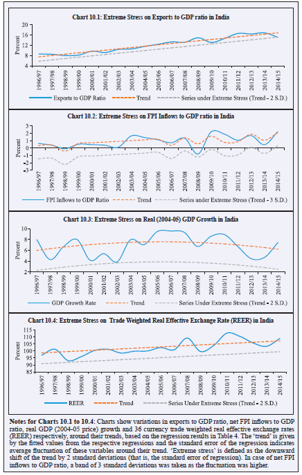

Simulation results

Table 5 summarizes the estimated parameters and shows optimum reserves under different crisis scenarios. In the Lehman type scenario, optimum reserves are estimated at 7.6 per cent of GDP for 2008-14 compared to the optimum reserves to GDP ratio of 9.1 per cent obtained by J&R. Chart 11 shows the optimum level of reserves under the Lehman type and extreme stress scenarios, and compares them with actual reserves. Optimum reserves in US$ billion are calculated by multiplying the reserves to GDP ratio by quarterly GDP levels.

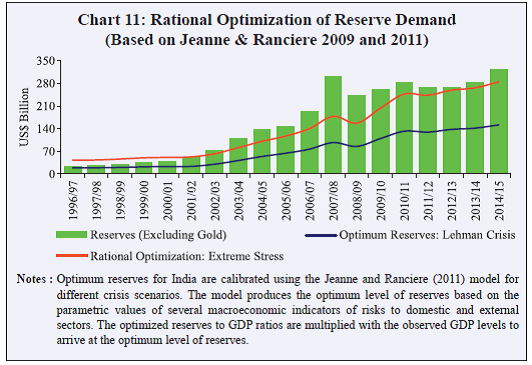The simulation results suggest that foreign exchange reserves in 2014-15 remained sufficiently above the level which could be optimum in a Lehman type crisis, and also an extreme stress scenario since 2003-04. As reserves are also estimated to be higher than the optimized level corresponding to most of the years, it could imply that the foreign exchange reserves in India may be considered ‘adequate’ to capture a broad set of potential risks to the country’s external sector.

Finally, Chart 12 compares the simulation results with predicted reserves from the econometric estimation. The optimum reserves under extreme stress remained lower than the predicted reserves from the regression (with a 2 SD band) since 2003-04, except in 2012-13 and 2014-15. Reserves’ demand as predicted by the econometric model was far in excess of the optimum level derived from the model under extreme stress; for the years around the global financial crisis – 2007-08 to 2009-10 -- which has moved closer since then. For example, in 2014-15, predicted reserves from the regression analysis were US$ 347 billion (with a 2 SD upper band), while the optimum reserves simulated under the extreme stress scenario were US$ 284 billion.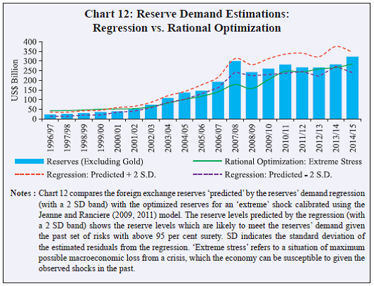

Actual reserve levels in 2014-15 were slightly higher than the levels derived from the theoretical model under extreme stress, and also within the range predicted by the regression model. Therefore, we held that the current stock of foreign exchange reserves in India may be adequate to cover potential risks to the external sector.

Section IV

Conclusion

This paper assessed the adequacy of foreign exchange reserves in India using different approaches. First, it observed that reserves in India are significantly higher than the levels in some other major economies with similar external sector characteristics. Second, an econometric analysis revealed that India’s actual reserve levels were within the adequacy band of 2 SD around the predictions from an estimated reserve demand equation. Finally, it calibrated a model for India based on Jeanne and Ranciere (2009, 2011) for optimum reserves’ demand under a Lehman type and an extreme stress scenario to suggest that actual reserves in India remained sufficiently higher to cover that stress. There were instances when actual reserves in India fell below adequate reserves as suggested by econometric models, but not by optimization models. It also observed that the econometrics model tends to suggest a somewhat higher level of optimal reserves for earlier years (2003-12), but both estimates tend to converge for the more recent years.

Although, India’s current reserve levels are adequate, it is important to examine the availability of various other foreign currency asset substitutes such as sovereign wealth funds, currency swaps and IMF’s contingency funds to augment its foreign exchange reserves position. As India has limited access to such asset lines beyond its currency swap agreements of US$ 50 billion with Japan a sufficient reserves buffer may be necessary to ensure against any perceived risk as also to ensure the stability of its external sector.

References

Aizenman, J. and N. Marion (2002), ‘The High Demand for International Reserves in the Far East: What’s Going On?’, NBER Working Paper No. 9266.

Anand, R., K.C. Cheng, S. Rehman and L. Zhang (2014), ‘Potential Growth in Emerging Asia’, IMF Working Paper/14/2, January.

Aziz, J. (2012), ‘Facing Falling Potential Growth’, The Economic Times, September 14. Available at: http://epaper.timesofindia.com

Bajpai, N. (2011), ‘Global Financial Crisis, its Impact on India and the Policy Response’, Working Papers Series, Columbia Global Centres, No. 5, July.

Chakravarty, M. (2013), ‘India’s new normal growth rate is 6-7%’, live Mint, , March 3. Available at: http://www.livemint.com

Chinoy. S. (2012), ‘RBI has made a very prudent move’, The Economic Times, , July 31. Available at: http://articles.economictimes.indiatimes.com

Dua, P. and A. Sinha (1997), ‘East Asian Crisis and Currency Pressure: The Case of India’, Working Paper, Centre for Development Economics, Delhi School of Economics, No. 158, August.

Edison, H. (2003), Are Foreign Reserves in Asia too High?, World Economic Outlook 2003 Update, Washington, DC: International Monetary Fund.

Flood, R. and N. Marion (2002), ‘Holding International Reserves in an Era of High Capital Mobility’, IMF Working Paper/02/62, April.

Ghosh, A., J. Ostry and C. Tsangarides (2012), ‘Shifting Motives: Explaining the Buildup in Official Reserves in Emerging Markets since the 1980s’, IMF Working Paper/12/34, January.

Gosselin, M.A. and N. Parent (2005), ‘An Empirical Analysis of Foreign Exchange Reserves in Emerging Asia’, Bank of Canada, Working Paper 2005-38, December.

Gourinchas, P.O. and M. Obstfeld (2012), ‘Stories of the twentieth century for the twenty-first’, American Economic Journal: Macroeconomics, 4(1): 226-265.

IMF (2011), Assessing Reserve Adequacy. February.

_______(2013), Assessing Reserve Adequacy-Further Considerations. Policy Paper, November.

Jeanne, O. and R. Ranciere (2006), ‘The Optimal Level of International Reserves for Emerging Market Countries: Formulas and Applications’, IMF Working Paper/06/229, October.

___________(2009), The Optimal Level of International Reserves for Emerging Market Countries: a New Formula and Some Applications. Johns Hopkins University Publications, February.

__________(2011), ‘The Optimal Level of International Reserves for Emerging Market Countries: a New Formula and Some Applications’, The Economic Journal, 121: 905–930.

Prabheesh, K. P., D. Malathy and R. Madhumathi (2009), ‘Precautionary and mercantilist approaches to demand for international reserves: an empirical investigation in the Indian context’, Macroeconomics and Finance in Emerging Market Economies, 2 (2): 279-291.

Mishra, P. (2013), Has India’s Growth Story Withered? New Delhi: Ministry of Finance, Government of India.

Mishra, R. and C. Sharma (2011), ‘India’s demand for international reserve and monetary disequilibrium: Reserve adequacy under floating regime’, Journal of Policy Modeling 33(2011): 901-919.

Park, D. and G. Estrada (2009), ‘Are Developing Asia’s Foreign Exchange Reserves Excessive? An Empirical Examination’, ADB Economics Working Paper Series, Asian Development Bank, No. 170, August.

Patnaik, I. and M. Pundit (2014), ‘Is India’s Long-term Trend Growth Declining?’, ADB Economic Working Paper Series, No. 424, December.

Prakash, A. (2012), ‘Major Episodes of Volatility in the Indian Foreign Exchange Market in the Last Two Decades (1993-2013): Central Bank’s Response’, RBI Occasional Papers, 33 (1 & 2).

Rai, V. and L. Suchanek (2014), ‘The Effect of the Federal Reserve’s Tapering Announcements on Emerging Markets’, Working Paper, Bank of Canada, No. 50.

Ramachandran, M. (2004), ‘The optimal level of international reserves: evidence for India’, Economics Letters, 83: 365–370.

Sehgal, S. and C. Sharma (2008), ‘A Study of Adequacy, Cost and Determinants of International Reserves in India’, International Research Journal of Finance and Economics, 20: 75-90.

Vasant and Jain (2012) ‘Subbarao: Potential Growth May Have Fallen’, The Wall Street Journal, July 17. Available at: http://www.wsj.com

Annexure I: Data

For the peer comparison, data on reserves is taken from the World Development Indicators (WDI) database of the World Bank, while the current account balance and nominal GDP, used to scale the reserves, are taken from the World Economic Outlook database of the IMF. Net foreign portfolio investment (FPI) inflows are used for a cross-country comparison, and are also taken from WDI. A cross-country comparison of India’s reserves with comparator countries uses annual data from 2001 to 2014.

The econometric estimation uses quarterly data on India’s foreign exchange reserves (excluding gold), nominal GDP at market price, imports, current earnings (credit item in current account), net foreign portfolio inflows in equity, 36 currency trade-weighted nominal and real effective exchange rates, broad money (M3) and the 91-day treasury bill rates for both India and the US. All the data for India are obtained from the Reserve Bank of India’s website except the 91-day Treasury bill rate for the US, which is taken from the website of the Federal Reserve. The estimation uses quarterly data from the first quarter (Q1) of the financial year 1996-97 (starting April 1996) up to the first quarter of 2015-16 (end-June 2015).

In order to calibrate the Jeanne and Ranciere (2011) model for India, the paper uses annual data for the period 1996-97 to 2014-15. The calibration exercise uses information on: (i) exports to nominal GDP ratio, (ii) net FPI inflows to nominal GDP ratio, (iii) real (2004-05 prices) GDP growth rate, and (iv) 36 currency trade-weighted REER depreciation. All data are taken from the Reserve Bank of India’s website.

Annexure II

Table 1.a: Phillips-Perron unit root test on the variables and estimated residuals of reserve demand regression

Table 1.a shows the results of the Phillips-Perron unit root test on the variables and the estimated residuals of the reserve demand regression (Table 2). * indicates rejection of the null hypothesis (H₀: ‘presence of unit root’) at 1 per cent level of significance. The test indicates that all the variables except the current earnings’ volatility are stationary (that is, absence of unit root) in their first difference. Current earnings’ volatility is stationary only at a 10 per cent level of significance. The estimated residuals are stationary at 1 per cent.

Table 1.b: Results of the Johansen co-integration test between the variables used in reserve demand regression

Table 1.b shows the results from the Johansen co-integration test between the reserve to GDP ratio and the variables of precautionary demand and opportunity cost. The test based on max-eigenvalue indicates that there exists at least one co-integrating relation between these variables. ***, ** and * indicate rejection of the null hypothesis at 1 per cent, 5 per cent and 10 per cent levels respectively.

* Rajib Das (email) and Siddhartha Nath (email) are Director and Research Officer respectively in the Department of Economic and Policy Research, Reserve Bank of India, Mumbai. The views expressed in the paper are those of the authors and do not necessarily reflect the views of the Reserve Bank of India. The authors thank the anonymous referee for valueable comments. The authors also acknowledge the guidance provided by Dr. Prachi Mishra and some suggestions offered by Pankaj Kumar from the Reserve Bank of India during the writing of the paper.

¹ Foreign portfolio investment (FPI) inflows indicate ‘net’ inflows, that is, gross inflows minus gross outflows, unless otherwise mentioned. The years denote financial years (from April-March). For FPI inflows, the comparison is between 2000-01 - 2007-08 and 2009-10 - 2014-15. 2008-09 is excluded as this was the year of the global financial crisis, when India had net FPI outflows.

² See Dua and Sinha (1997), Bajpai (2011), Rai and Suchanek (2014) for contagion effects of external shocks on the Indian economy.

³ See Prakash (2012) for a detailed survey of the steps taken by RBI during major episodes of volatility in the Indian foreign exchange market over the last two decades.

⁴ The paper does not cover the period before 1996-97 as the Indian rupee has been market determined only since then (with the currency regime broadly characterized as a managed float without any pre-determined bands). Prior to that, changes in stock reserves were determined only by the need to maintain a particular level of the exchange rate.

⁵ See Ghosh et al. (2012) for a survey of literature on motives behind reserve holdings.

⁶ See IMF (2011), Ghosh et al. (2012).

⁷ FPI inflows in public and publicly guaranteed and private non-guaranteed bonds are not available for all the countries in the sample. Therefore, only FPI in equity is reported and used in this exercise.

⁸ See, for example, Gosselin and Parent (2005) and IMF (2011).

⁹ The ceiling for FPI in government securities and corporate bonds was US$ 10 billion and US$ 40 billion in 2010, which was subsequently increased to US$ 30 billion and US$ 51 billion, respectively.

¹⁰ The Phillips-Perron test for unit root shows that reserves to GDP, imports to GDP, nominal effective exchange rate, current earnings’ volatility, FPI inflows’ volatility, broad money to GDP ratio, REER undervaluation and interest spread between India and US on 91-day treasury bills were all non-stationary in their levels, however, they were stationary in their first differences (Table 1a in Annexure II). The estimated residuals from estimating Equation 1 are stationary in levels, indicating presence of co-integration among the variables. Johansen test also confirms the existence of co-integration among these variables (Table 1.b in Annexure II).

¹¹ Jeanne and Ranciere (2011) do not account for valuation change in external payments due to currency depreciation and hence, do not include the parameter. This paper follows Jeanne and Ranciere (2009) instead, and also accounts for currency volatilities, which are relevant for India.

¹² FPI in both debt and equity are used.

¹³ J&R define a year of ‘sudden stop’ as one with a more than 5 percentage points decline in the capital inflows to GDP ratio over the previous year. In the Indian context, this paper uses the terms ‘crisis years’ instead of sudden stops.

¹⁴ J&R averaged the estimated probabilities across all the years to arrive at a constant parametric value of π. This paper, however, allows the probability of crisis to vary over time, as the global circumstances and the external sector fundamentals in India have changed significantly since the late 1990s.

¹⁵ Net FPI inflows declined to US$ 9 billion in 2013-14, compared to US$ 30 billion, US$ 32 billion, US$ 19 billion and US$ 31 billion in 2009-10, 2010-11, 2011-12 and 2012-13, respectively. It increased to US$ 46 billion in 2014-15.

¹⁶ See, for example, Anand et al. (2014), Patnaik and Pundit (2014), Mishra (2013), Vasant and Jain (2012), Chakravarty (2013), Aziz (2012) and Chinoy (2012).