Suman Yadav and Ravi Shankar* Expectations about consumer inflation play an important role in individual consumption and saving decisions leading to differing macroeconomic outcomes. The major economic variables that shape individual spending decisions include income and inflation/inflation expectations. In India, inflation and expectations about it have persisted at relatively higher levels in the recent period and may be one of the major factors influencing households’ spending decisions. This study presents the empirical relationship between inflation expectations and consumers’ spending in India using micro-data from the Reserve Bank of India’s quarterly Consumer Confidence Survey of households. We found that higher inflation expectations lead to higher current household spending and also to planning for reduced spending in the future. These findings are found to be stable over time and across various demographic and individual attributes. JEL Classification : D10, D91, E20, E21, E30, E31 Keywords : Expenditure, Households, Spending, Inflation Expectation, Inter-temporal Consumer Choice Introduction Consumer spending emanating from economic decisions of more than 200 million households in India forms a major portion (about 60 per cent) of GDP as private final consumption expenditure. Consumers’ purchase choices affect not only the aggregate size of the economy but also influence prices and inflation, making it pertinent to examine households’ inflation expectations and their relationship to consumer spending. Understanding this relationship can provide useful inputs for monetary policy. Changes in the expected inflation rate are said to force consumers to alter their planned expenditure programmes and reallocate spending - current or future. Traditional micro-models of consumer spending consider a trade-off between consumption and saving. An expected increase in prices results in shifting planned future spending to the current period. Higher expected inflation also lowers the real interest rate, which leads to lower returns, less savings and thus more current spending. On the other hand, higher inflation creates uncertainties about the future which can cause downward revision in real income expectations leading to lower current consumer spending (Juster and Wachtel 1972). The exact direction of this relationship is important for macroeconomic policy. For instance, researchers like Eggertsson and Woodford (2003) and Krugman (1998) have argued that central banks should commit to policies that raise expectations of future inflation, thereby affecting a decline in real interest rates and encouraging greater current spending. This viewpoint suggests that purchases of large consumer durables and residential housing, purchases that are readily substituted across time and that are often financed with debt, should be particularly sensitive to an increase in expected inflation. Microeconomic data are needed to identify a causal relationship between individual household inflation expectations and spending behaviour. Some studies have examined the relationship between inflation expectations and consumer spending using microeconomic data. Based on data from the University of Michigan’s Survey of Consumers, Bachmann et al. (2015) observed no significant relationship between inflation expectations and the ‘readiness to spend’ on durable goods. The study found that higher expected inflation has an adverse impact on the propensity to spend. While average ‘readiness to spend’ is observed to be correlated with aggregate spending in the National Income and Product Accounts (NIPA) (a part of the national account in the United States), there is little evidence of a relation between individuals’ readiness to spend and individual spending. Ichiue and Nishiguchi (2013) employed data on actual over-the-year spending changes and planned one-year-ahead spending changes. Using data from Bank of Japan’s Survey on Consumer Opinions, they found that respondents with higher inflation expectations tended to indicate that their household real spending had increased over a year back levels and they expected decreased future spending. This relation is observed to be stronger for financial asset holders. Both these studies identified effects using variations in behaviour across households rather than variations within households over time. Thus the studies cannot control for unobserved heterogeneity among households. Burke and Ozdagli (2013) revisited the relationship between household inflation expectations and consumer spending by using panel survey data from New York Fed/RAND for April 2009 to November 2012. The panel dimension of the data allowed controlling for unobserved heterogeneity at the household level. They found that promoting higher inflation expectations may be insufficient for boosting current consumer spending. Additionally, in some cases an increase in inflation expectations created a negative income effect that discouraged spending in both the present and in the future. The heterogeneity in findings based on the method used and on geography motivates our study. In this paper we examine the relationship between inflationary expectations and consumer spending in India during 2011-14. Indian evidence provides an interesting motivation because nominal interest (on 1-3 years deposits) was around 8.25–9.25 per cent (RBI 2014-15) while the inflation rate was about 8.4–10.4 per cent (average CPI-IW) leading to low real interest rates. This is in contrast to low nominal and positive real rates in developed economies. In this economic backdrop, households in India need to balance their current consumption and aspired future consumption. The negligible coverage of social safety nets in India further complicates household consumption decisions. Given this scenario, it is interesting to look at consumer behaviour in India even as not many studies have been done covering this aspect. Hence, this study fills an important gap in behavioural consumer studies in India given the availability of consumer survey data in recent times. This study used micro-data from the Reserve Bank of India’s (RBI) quarterly Consumer Confidence Survey (CCS) from March 2011 to September 2014. The survey data provide valuable insights into urban consumer behaviour. For an analytical framework this study used the established framework used by Ichiue and Nishiguchi (2013) in the absence of any better alternative in the Indian economic context. By using an established framework, the study may not contribute in terms of technique but it adds to knowledge on Indian consumer behaviour as the analysis is based on a technique used earlier. The rest of the paper is organised as follows: Section II presents a review of relevant literature. Section III describes the data used for analysis and Section IV explains the methodology. The results are given in Section V while Section VI addresses robustness checks. Section VII provides a conclusion. Section II
Literature Review There are three main theories of consumption and saving: (i) the life-cycle hypothesis (Ando and Modigliani 1963; Modigliani and Ando 1957; Modigliani and Brumberg 1954); (ii) the permanent income hypothesis (Friedman 1957); and (iii) the relative income hypothesis (Duesenberry 1949). The life-cycle and permanent income hypotheses are the most popular which are also relatively similar; both theories assume that individuals attempt to maximize their utility or personal well-being by balancing a lifetime stream of earnings with a lifetime pattern of consumption. Many studies have tried to establish the existence of a stable relation between consumption, income and other relevant variables and to estimate its parameters. Such relations are useful tools for economic policy and forecasting. During the last few years, research work in this area has mainly taken two directions. The first characterizes a correlation of data on aggregate consumption or saving with income and several other control variables, and the second direction exploits cross-sectional data. Juster and Wachtel (1972) investigated the relationship between consumer spending, inflation and inflation expectations. Using aggregate time-series data on spending and inflation expectations, they found that higher inflation expectations led to lower spending on durable goods and an increase in savings. They also found that inflation increased consumer spending on non-durables and services. Springer (1977) studied the effect of inflation expectations on consumer expenditure and found that consumers reallocated expenditure in response to the expected rate of inflation. His results show that the expected rate of inflation has a consistently negative impact on expenditure on non-durables and services. Bernanke (1981) studied consumer purchases of non-durables and durables as the outcome of an optimisation problem. He found that the presence of adjustment costs of changing durable stocks may substantially affect the time-series properties of both components of expenditure under the permanent income hypothesis. Zeldes (1989) tested the permanent income hypothesis against the alternative hypothesis that consumers optimize their consumption subject to a well-specified sequence of borrowing constraints. He derived implications for consumption in the presence of borrowing constraints. His tests used time-series (cross-section) data on families from the University of Michigan’s Panel Study of Income Dynamics. The results support the hypothesis that an inability to borrow against future labour income affected the consumption of a significant portion of the population. Armantier et al. (2011) compared inflation expectations reported by consumers in a survey with their behaviour in a financially incentivized investment experiment in which the inflation affected the final payoff. The authors also found that decisions taken by the respondents in the survey were on average consistent and under risk neutrality with their stated inflation beliefs. Wiederholt (2012) showed that in a model with dispersed information, a commitment by policymakers to higher inflation may send negative signals about the future outlook for the economy thereby reducing current consumption. A recent study by Arnold et al. (2014), using micro-data from the second wave of the Hamburg-BUS Survey (Germany), evaluates the link between consumer saving portfolio decisions and inflation expectations. They analysed whether consumers respond to their own inflation expectations and economic news that they have observed recently while planning to adjust their saving portfolios in the next year. Their results reveal that higher inflation expectations only affected planned saving adjustments due to a higher interest rate. This is in line with the results of Bachmann et al. (2015) and Burke and Ozdagli (2013) regarding the relation between consumers’ inflation expectations and consumption. However, Ichiue and Nishiguchi (2013) observed opposite results for Japanese consumers. Section III
Data Description Micro-data from RBI’s CCS, with quarterly frequency form the basis for this study. The survey obtains information on urban consumer sentiments and is published regularly on the RBI website.1 The RBI survey has been conducted since June 2010. For each round of the survey 5,400 respondents, aged 21 years and above from different households are canvassed in six metropolitan cities of Bengaluru, Chennai, Hyderabad, Kolkata, Mumbai and Delhi. The survey fieldwork is subjected to rigorous quality checks through on-site/off-site verifications and hence the total responses included in the study may not always add up to the targeted sample size. The respondents are selected in a way to ensure randomness in the sampling design. Each city is divided into three major areas and each major area is further divided into three sub-areas. From each sub-area, about 100 respondents are selected randomly. In each round of the survey, 5,400 respondents are selected (900 respondents from each city). Details about the survey are available on the RBI website.2 The RBI survey captures qualitative responses on questions pertaining to economic conditions, household circumstances, income, spending, prices, employment prospects and other economic indicators. The responses are in two parts -- the current situation as compared to a year ago and expectations for a year ahead. From Q2:2012-13 onwards, the survey schedule has been modified to include perceptions on future household circumstances, outlay for major expenditures (motor vehicles, house, consumer durables, etc.), the current employment scenario and current/future rate of price increase. The qualitative responses are obtained on a three-point scale -- positive/no change/negative. The survey also contains rich demographic information on the respondents, including information on sex, age, geographic location, family size, annual income and employment status. All these responses are used as control variables in our analysis (see Annexure I for the survey questionnaire). The survey captures respondents’ expectations on prices and household spending. Thus, we can match spending with inflation expectations from the same source response. Further, the respondents (only one response from a household) need not necessarily be the head of the family, and so the survey response represents consumer views of individuals (both head of family and future head of family). In this study we mainly focus on individual responses to two questions: Q1: How have you (or other family members) changed consumption spending compared to one year ago? and Q2: In which direction do you think prices will move one year from now? Responses to current spending (Q1) take on three different qualitative options: Increased, remained the same and decreased, while responses to prices (Q2) are categorized as ‘will go up’, ‘will remain the same’ and ‘will go down’. We also included a model with perception on current spending and perception on price levels compared to one year ago. The response-level micro-data from the March 2011 round to the latest round (September 2014) are used for our study. This gave us a fairly large number (about 77,000) of observations. The broad features of the consumer survey data used in this analysis are already published in the RBI Bulletin (September 2013 and September 2014 issues) and so are not presented here. The basic features of the dataset used, however, are presented in Annexure II. Section IV
Empirical Set-up and Methodology This section presents the empirical set-up and methodology used for the study. To examine the relationship between inflation expectations and consumer spending, we used two models following the approach adopted by Ichiue and Nishiguchi (2013). The dependent variables were responses to questions about changes in expected future spending and actual current spending respectively. The first model was used to study whether high inflation expectations led to a lower expected change in real future spending (inter-temporal substitution effect). The second model was used to examine whether higher inflation expectations led to greater real current spending. We used an ordered probit model as the responses were categorical and ordered. IV.1 Expected Change in Real Spending In this sub-section we construct a baseline specification for examining the relationship between inflation expectations and the expected change in real spending for the next year. In standard Dynamic Stochastic General Equilibrium (DSGE) models the key equation is the Euler equation derived from the optimisation problems of households. The main results state that real interest rates and expected real consumption growth rates are correlated. Therefore, a lower interest rate creates an incentive for consumers to reduce their savings resulting in more spending now rather than in the future (Baba 2000; Hamori 1992, 1996; Nakano and Saito 1998). Bachman et al. (2013) studied the empirical relationship between expected inflation and spending attitudes using micro-data from the Michigan consumers’ survey. They found negative results for this relationship which is contrary to the standard DSGE models. Ichiue and Nishiguchi (2013) observed that the respondents with higher inflation expectations tended to indicate that their households had increased current real spending (compared to one year ago) but would decrease it in the near future. Both studies pertain to developed economies with lower interest rates or a zero interest rate. We aim to study the relationship between expected inflation and spending attitudes of Indian consumers and whether the results obtained by Ichiue and Nishiguchi (2013) hold true for consumers in a developing economy like India. We took the CCS data which captures nominal spending rather than real spending. Following Ichiue and Nishiguchi (2013) we constructed responses to an artificial question about the expected change in real spending in the next year by synthesizing the responses on two questions about inflation expectations: Question 14 in the CCS questionnaire and expected changes in nominal spending (Question 9 in the CCS questionnaire): Q9: Do you plan to increase or decrease your spending within the next 12 months? -
Increase -
Neither increase nor decrease -
Decrease Q14: In which direction do you think prices will move one year from now? -
Will go up -
Will remain almost unchanged -
Will go down • First we associated each response to these two questions with a real number according to its contribution to nominal spending and prices to real spending. For the spending question (Q9), the responses -- increase, neither increase nor decrease and decrease -- were graded as +1, 0 and -1 respectively. For price inflation (Q14), ‘will go up’ was graded as -1, ‘will remain unchanged’ as 0 and ‘will go down’ as +1. We considered both variables -- expectations on future spending and inflation increase/decrease. We defined real spending as: Real spending = Expected nominal spending - expected inflation | | Expectation on inflation in the next year (Q14) | | Increase | Same | Decrease | | Expectation on spending in next year (Q9) | Increase | Same | Increase | Increase | | Same | Decrease | Same | Increase | | Decrease | Decrease | Decrease | Same | The responses to the synthesized real spending question were then defined as ‘increase’ if the total sum was 1 or more; ‘remain the same’ if the sum was 0; ‘decrease’ if the total sum was -1 or less. These synthesized responses of real spending were used as a dependent variable in the ordered probit model. In the probit model the independent variables of interest are dummies regarding the answer to the question on expected inflation in the next year. We used dummies for answers ‘increase’ and ‘decrease’ only. The respondents who answered ‘remain the same’ were used as the reference group. Each dummy took a value 1 for the corresponding answer and 0 otherwise. We wanted to see whether the inter-temporal substitution effect was present or not. If the inter-temporal substitution effect existed then it is expected that the coefficient of the dummy ‘increase’ would turn out to be negative and vice versa. IV.2 Actual Change in Current Real Spending This constructed dependent variable was used to examine whether households which expected higher inflation tended to spend in the present rather than in the future. Even if the results supported this relation, we cannot say that an increase in the current spending of a household was due to its higher inflation expectation. For instance, an income effect can dominate the inter-temporal substitution effect. Equivalently, households may not expect a change in income in line with an expected change in inflation due to which they may decrease spending. Moreover, the change, that is, decrease may be smaller than that in future spending due to the substitution effect. Another possibility is that many households do not allocate their spending inter-temporally in a rational manner but just follow a simple rule to stabilize their nominal spending. Such households may expect that their real spending will decrease just by the rate of increase in the price level, and their current spending is not influenced by the expected inflation rate. Keeping these possibilities in mind we constructed a second model to examine whether higher expected inflation led to an increase in real current spending as compared to one year ago. The dependent variable in the second model is responses to the question about the actual change in real spending. The dependent variable of Model 2 was synthesized using the following questions: Q7: How have you (or other family members) changed consumption spending compared to one year ago? -
Increased -
Remained the same -
Decreased Q12: How do you think the overall prices of goods and services have changed compared to one year ago? -
Gone up -
Remained almost unchanged -
Gone down We define real spending as: Real current spending = Expected nominal current spending – perception on inflation | | Perception on inflation compared to a year ago (Q12) | | Increase | Same | Decrease | | Perception on spending compared to one year ago (Q7) | Increase | Same | Increase | Increase | | Same | Decrease | Same | Increase | | Decrease | Decrease | Decrease | Same | Using the same methodology as in the first model, responses of the dependent variable for the second model were constructed. The main independent variables continued to be the dummies for inflation expectations. Although the main independent variables were identical to those in specification 1, the expected signs on the coefficients in specification 2 were the opposite of those in specification 1. The reason for this is that higher expected inflation leads to a higher level of current spending and this is likely to lower the expected change in real spending and to raise the actual change (magnitude) compared to one year ago. IV.3 Methodology Due to the categorical nature of the data the conventional linear regression specification was inappropriate. Therefore, like Ichiue and Nishiguchi (2013), we also used an ordered probit model which assumes that there is an unobserved variable for each observation i. The expected change in real spending can be modelled as: with threshold values α1 and α2, using the maximum likelihood estimation procedure we estimate the ordered probit model as well as threshold values. In the probit model discussed earlier the main independent variables of interest are dummies for the response to the question on expected inflation in the next year. We used two dummies for answers ‘increase’ and ‘decrease’. The respondents who answered ‘remain almost unchanged’ were used as a reference group. Each dummy took value 1 for the corresponding answer and 0 otherwise. We wanted to see whether the inter-temporal substitution effect was present or not. If the inter-temporal substitution effect existed then it was expected that the coefficient on the dummies for ‘increase’ would be negative and that for ‘decrease’ would be positive. To be able to interpret the coefficient on the dummies as the ‘causal’ effect to inflation expectations and spending, the regression specification needs to control for other determinants of spending which may be correlated with inflation expectations. These covariates can be either cross-sectional or aggregate in nature. Certain demographic characteristics are correlated with both spending attitudes and inflation expectations. The vector of control variables, therefore, includes a set of demographic factors also. The CCS households collects many demographic characteristics of respondents. The vector of variables for individual attributes includes dummies for gender, age-group, occupation, annual income levels of the households and family size. The first item in the list of each set of dummies is treated as the reference group. The survey is conducted in six metro cities and so we included dummies for cities also taking Delhi as the reference group. There may be other cross-sectional covariates imperfectly related to demographics which are also correlated with both inflation expectations and spending attitude. CCS has a rich set of information on idiosyncratic expectations and attitudes for which we can control in our regression models. A set of idiosyncratic expectations (qualitative) about idiosyncratic situations -- expectations and perceptions about the general economic situation, household circumstances, income and employment -- covered in the survey were used in the analysis. The responses for real income were constructed in a manner similar to the responses to the question about expected changes in real spending from the responses to the question on expected change in nominal income (Q6) and about inflation expectations. Next, we included idiosyncratic general economic conditions referring to the overall economic condition of the country as a whole (Q2) and expected (qualitative) changes in employment perceptions (Q11ii). Answers to all these questions were recorded on a three-point scale - ‘will improve/increase’, ‘remain the same’ and ‘will worsen/decrease’ and so two dummies were included for responses ‘will improve/increase’ and ‘will decrease/worsen’ taking the response ‘remain the same’ as the reference group. The inclusion of these two groups of dummies deals with the optimist/pessimist problem, that is, the fact that some people, for instance, are inherently optimistic and might, on average, expect an improvement in economic conditions, increases in real incomes and spending and decline in the prices of items planned for purchase. Thus, unless idiosyncratic expectations were controlled for, the estimated relationship between expected inflation and expected spending may be biased. Further, the inclusion of the dummies for idiosyncratic expectations of aggregate conditions also aims to deal with the potential endogeneity problem, that is, respondents who expect a strong economy may also expect increase in both price levels and spending. In such cases, the negative effect of expected inflation on the expected change in real spending may be underestimated unless this effect is controlled. In addition to this control vector, in the second ordered probit model (referred to as Model 2 in the rest of the paper) where the dependent variable is responses to perceptions on current real spending, we included dummies corresponding to perceptions on current levels of prices, current economic conditions, change in current employment, change in real current income (constructed using actual nominal income (Q5) and perception on inflation for current period (Q12)); household circumstances (Q4i) and change in current prices (Q12). Section V
Empirical Results An analysis was done using SAS as well as Stata software and we got similar results with both. Empirical results obtained from the two main models used for examining the relationship between inflation expectations and spending are now discussed. V.1 Main Results The estimated coefficients for the dependent variable on spending from the two models are given in Table 1 for economic/idiosyncratic expectations and in Table 2 for demographic controls. Table 1 shows that for both Models 1 and 2, all four coefficients estimated for expected inflation have the expected signs and are significant at the 1 per cent level, that is, respondents who expect higher inflation are more likely to indicate that their households will decrease real spending in the next year, and their households had increased real current spending compared to one year ago. In terms of economic control variables, the estimated coefficients of dummies for most of the control variables were found to be significant at a 1 per cent significance level with plausible signs. This gives us confidence that CCS is able to capture the underlying economic variables of interest reasonably well. Model 1: Expected Real Spending For Model 1, the dummies related to responses on expected changes in real incomes of households, expected employment scenario and expected changes in economic conditions had a positive relationship with expected changes in real spending, that is, the respondents who perceive ‘improvement’ for a control variable (as compared to reference) will expect an increase in future spending and for a ‘worsening’ response, they expect decreased future spending (Table 1). | Table 1: Estimation Results for Baseline Specifications | | Dependent variables | Real spending one year from now (Model 1) | Real spending compared to one year ago (Model 2) | | Prices one year from now | | | | Increase | -1.395* (0.02) | 0.770* (0.02) | | Decrease | 0.941* (0.03) | -0.306* (0.03) | | Prices compared to one year ago | | | | Increase | | -1.956* (0.03) | | Decrease | | 0.843* (0.04) | | Economic conditions one year from now | | | | Improve | 0.206* (0.01) | 0.174* (0.02) | | Worsen | 0.007 (0.01) | 0.201* (0.02) | | Economic conditions compared to one year ago | | | | Improve | | 0.067* (0.01) | | Worsen | | 0.043** (0.02) | | Household circumstances compared to one year ago | | | | Better | | 0.289* (0.02) | | Worse | | 0.117* (0.01) | | Real income one year from now | | | | Increase | 0.554* (0.03) | 0.511* (0.03) | | Decrease | -0.476* (0.01) | -0.530* (0.01) | | Real income compared to one year ago | | | | Increase | | 0.917* (0.04) | | Decrease | | -0.486* (0.02) | | Employment scenario one year from now | | | | Improved | 0.175* (0.01) | 0.027*** (0.01) | | Worsen | -0.100* (0.01) | -0.158* (0.01) | | Threshold | α1 = -1.644* (0.04) | α1 =-1.367* (0.04) | | | α2 = 0.935* (0.03) | α2 =2.184* (0.05) | | Number of observations: 75,573 | | Pseudo R2 : | 0.224 | 0.264 | | Note: *** ,** and * denote significance at the 10, 5 and 1 per cent levels respectively. Standard errors are in parentheses. | Dummies related to responses on expected changes in overall economic conditions have a positive sign for both types of responses - ‘improve’ or ‘worsen’ -- but the effects for the response ‘worsen’ dummy are insignificant indicating relatively muted distinction by Indian consumers on this question. Further, all other dummies for demographic control variables, (except age-group and annual income dummies in case of current spending), have significant effects on expected changes in spending indicating the importance of these aspects in expected consumer spending in India.3 | Table 2: Estimation Results for Baseline Specifications: Demographic Controls | | Dependent variables (with three dummies): | Real spending one year from now (Model 1) | Real spending compared to one year ago (Model 2) | | Independent Variables | Coefficients | Coefficients | | Gender | | | | Male | 0.006 (0.01) | -0.044* (0.01) | | Age-group | | | | 22-60 | 0.039*** (0.02) | 0.010 (0.02) | | Occupation | | | | Employed | -0.057* (0.01) | -0.041* (0.01) | | Annual income | | | | Up to ₹1 lakh | -0.059* (0.01) | -0.002 (0.01) | | Family size | | | | Up to 2 members | -0.066* (0.02) | -0.147* (0.02) | | 3 or 4 members | -0.004 (0.01) | -0. 084* (0.01) | | City | | | | Bengaluru | 0.485* (0.02) | -0.006 (0.02) | | Chennai | 0.061* (0.02) | 0.278* (0.02) | | Hyderabad | 0.248* (0.02) | 0.340* (0.02) | | Kolkata | 0.271* (0.02) | 0.410* (0.02) | | Mumbai | 0.399* (0.02) | 0.099* (0.02) | | Note: See the notes to Table 1. Demographic controls include the dummy which takes unity for female respondents and 0 for males (sex) ; dummy which takes unity for respondents age less than or equal to 60 years and 0 otherwise; dummy which takes unity for employed respondents and 0 otherwise. Moreover a dummy which takes value 1 for respondents’ family size is less than or equal to 4 and 0 for family size greater than 4. | Model 2: Real Current Spending A change in real current spending (Model 2) has a negative relationship with current perceptions on prices whereas the relationship is positive with inflation expectations. These results also reinforce the results obtained in Model 1 indicating that Indian consumers do not intend to increase future spending with an increase in prices (Table 1). The coefficient dummies of responses on economic control variables, that is, economic conditions, household circumstances, real incomes of households and expected employment scenario are significant and have a positive relation with changes in current spending. It is observed that the contribution of expected inflation as well as other control variables is relatively small in Model 2 as compared to Model 1. The coefficients in Model 2 are of a smaller magnitude (absolute value) than those in Model 1. As observed by Ichiue and Nishiguchi (2013), one plausible reason for lower coefficients for Model 2 could be the presence of effects other than the inter-temporal substitution effect. Model 1 is designed to estimate only the substitution effect but not adverse effects such as the income-effect. Model 1 is likely to overestimate the total impact of expected inflation on current spending due to its construction. Additionally, Model 1 may suffer from the 'measurement error’ associated with expected future changes which are natural for individual respondents. Model 2 is free from a possible estimation bias discussed earlier mainly due to three reasons. Firstly, respondents are asked about the 'actual/observed changes’ in nominal spending compared to one year ago in Q7, similar to the wording of Q12, about the 'actual changes’ in prices. Secondly, the dependent variable is constructed using the question about the actual changes in prices, while the main independent variables are dummies about the expected changes in prices. Because of this difference, Model 2 suffers less from any potential measurement error of expected inflation. Thirdly, the Model 2 specification uses responses on currently observed inflation to construct both the dependent and independent variables. Thus, even if the dependent variable is biased by construction due to over or underestimation of the effect of actual change in prices on real spending, the estimation bias of the coefficients on expected inflation should be limited because it is absorbed into the coefficients on actual inflation. Model 2 is expected to underestimate the impact of expected inflation on real current spending since it uses the constructed response rather than the survey response on current spending as the dependent variable. If expected inflation (one year ahead) rises then, both the level of current real spending and the actual spending growth rate is expected to increase. However, if higher inflation (one year ahead) was already expected one year ago, current spending may still be greater but the actual growth from one year ago to now need not necessarily be higher, since past spending may also have been greater. Because of this possibility, the impact of expected inflation on increased spending is expected to be smaller than that on current spending. Section VI
Robustness Checks In the first sub-section, we check the robustness of results by changing the dependent variable. We used nominal spending instead of real spending as the independent variable to examine whether the method of constructing real spending affected the results. The results presented in sub-section VI.1 give the robustness of Model 2. Further, sub-sections VI.2 and VI.3 present sub-sample analyses to examine whether the results from Models 1 and 2 remain unchanged even in sub-samples. Specifically, sub-section VI.2 uses sub-samples of each wave (round) of the survey, while sub-section VI.3 uses sub-samples by individuals’ attributes. As discussed earlier, both dependent variables in probit models have some biasness in results due to their construction methodologies. Therefore, in sub-section VI.4 we used another variable, relative spending growth, which is free from such biases in Model 2, to check the relationship. Sub-section VI.5 describes the relationship between real actual change in spending, actual inflation and Real Private Final Consumption Expenditure (RPFCE). As discussed before, the dependent variable is biased by construction due to over or underestimation of the effect of actual change in prices on real spending. An attempt has been made to reduce this bias by taking five dummies (five-point scale instead of three-point scale) for responses on real spending and examine the relationship between spending and inflation expectations. The results are presented in Annexure III which is in line with earlier results. VI.1 Nominal Spending In this sub-section we examine whether our definition of real spending leads to any bias in estimates by comparing results from the alternate ordered probit model. Both base Models 1 and 2 use the constructed ‘real’ spending response instead of actual response on spending which is unadjusted for inflation response. As discussed earlier, Model 2 seems to be free from possible estimation biases as it uses responses to current (actual) inflation to construct dependent real spending and also as a control variable. We used survey responses about actual change in nominal spending (Q7) as the dependent variable instead of changes in real spending used in Model 2. Moreover, in place of constructed ‘real income’ of a household, nominal income, that is, the actual survey response on households’ incomes is used as control variable. Table 3 shows that the inflation expectations have a statistically significant positive relation with nominal spending also. | Table 3: Estimation Results for Baseline Specifications with Actual Nominal Spending | | Dependent variables: | Nominal spending compared to one year ago | | Prices one year from now | | Increase | 0.250* (0.02) | | Decrease | -0.074** (0.03) | | Note: ** and * denote significance at the 5 and 1 per cent levels, respectively. Standard errors are in parentheses. |
| Table 4: Estimation Results for Baseline Specifications with Actual Nominal Spending | | Dependent variables: | Nominal spending compared to one year ago
(real income as control variable) | | Prices one year from now | | Increase | 0.682*(0.02) | | Decrease | -0.270* (0.03) | | Note: * denote significance at the 1 per cent level. Standard errors are in parentheses. | This positive relation was observed to be stronger if we used response on current and expected real incomes of households’ as control variables instead of nominal income (Table 4). Note that if we had used the responses on expected nominal spending changes as the dependent variable and we found that higher expected inflation led to a higher expected change in nominal spending, we could not have distinguished whether higher expected inflation leads to a higher expected change in real spending or in nominal terms only. On the other hand, where the current nominal spending growth is taken as the dependent variable, we can easily identify the effect of inflation expectations as the dependent variable ‘current spending’ and the main independent variable ‘inflation expectations’ are for different time periods. VI.2 Sub-sample Analysis over Time This sub-section presents robustness of the relationship between inflation expectations and consumers’ spending over time. While pooling cross-sectional data across time, one might be concerned about variations in the results obtained across time. The trend variation over time may tend to show a relationship between inflation expectations and consumers’ spending growth positively, even when it is negative. Therefore, we worked out main results over time as an additional check for robustness. For this purpose, data from each survey round were used as a sub-sample for estimating Models 1 and 2. Obviously, time dummies were not used as a control variable in these models. Charts 1 to 4 display the estimates for dummies regarding expected inflation for each survey round, together with 95 per cent confidence intervals. Charts 1 and 2 show that the negative relation between inflation expectations and expected changes in consumers’ spending is stable over time. That is, the point estimates of Model 1 shown in the charts have the expected signs for both inflation expectation dummies in all survey rounds, although they are insignificant in some survey rounds. Charts 3 and 4 show a positive relationship between inflation expectations and actual changes in consumers’ spending when they are significantly different from zero. These results are consistent with the full sample results giving confidence about the main results. 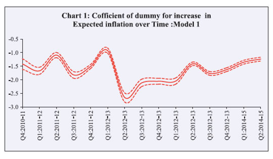 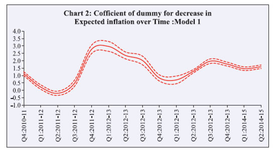 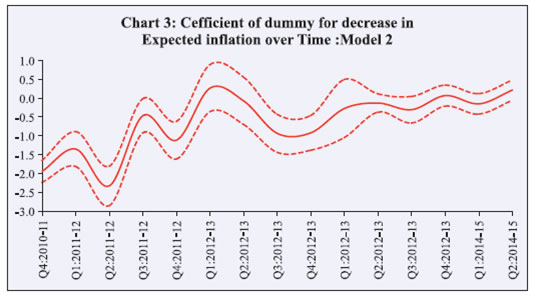 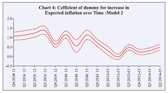 VI.3 Sub-sample Analysis with Effects of Individual Respondents’ Attributes It is generally expected that socioeconomic and demographic attributes effect individuals’ perceptions and expectations on prices and spending. For example, older/retired people are more likely to economize rather than spend as they are dependent on fixed rate incomes and thus their spending may be more influenced by inflation expectations. This sub-section investigates whether the relationship between inflation expectations and changes in spending are affected by the social and demographic attributes of the respondents. We considered demographic attributes like gender, age, annual incomes of households, family size, employment status and location of respondents. For this analysis, the whole sample was divided into two sub-samples according to the attributes of the respondents and then Models 1 and 2 were estimated for these sub-samples separately. For seeing the effect of age, respondents aged ‘60 years and above’ were taken in one group while the rest formed the other group. To examine our results across employment status the sample was divided into two groups: One group of employed respondents and the other of unemployed respondents. We also examined our results across household attributes like size and income. A household was small if the total number of members was 2, medium if it had 2-4 members and large if it had more than 4 members. Similarly, for household income, we divided the sample into two sub-samples - if the annual household income was ‘up to ₹5 lakh’ it formed one group and if the household income was ‘5 lakh and above’ it formed the other group. India being a large and diverse country it has considerable variations in production and consumption patterns across geographic regions and these variations are also reflected in price inflation due to local demand-supply factors. Therefore, we examined the main results over the geographical locations of respondents. The survey was conducted in six metros hence the sample was divided into six sub-samples according to the location of the respondents. The coefficients for the two models were estimated separately for these six sub-samples. The estimation results from the 15 sub-samples are given in Table 5. | Table 5: Sub-sample Analysis by Individual Attributes | | Dependent variable: | Real spending one year from now | Real spending compared to one year ago | | Prices one year from now: | Increase | Decrease | Increase | Decrease | | Gender | | Female | -1.389* (0.03) | 0.992* (0.05) | 0.731* (0.03) | -0.671* (0.05) | | Male | -1.440* (0.03) | 1.439* (0.06) | 0.689* (0.04) | -0.679* (0.07) | | Age-group | | 22 -60 | -1.406* (0.02) | 1.126* (0.04) | 0.728* (0.02) | -0.705* (0.04) | | 60 and above | -1.355* (0.08) | 1.265* (0.12) | 0.590* (0.08) | -0.330** (0.14) | | Occupation | | Employed | -1.382* (0.03) | 0.954* (0.05) | 0.748* (0.03) | -0.712* (0.06) | | Unemployed | -1.450* (0.03) | 1.422* (0.06) | 0.666* (0.03) | -0.617* (0.06) | | Annual income | | Up to ₹1 lakh | -1.288* (0.03) | 1.081* (0.05) | 0.682* (0.03) | -0.538* (0.06) | | ₹5 lakh and more | -1.481* (0.03) | 1.150* (0.05) | 0.735* (0.03) | -0.850* (0.06) | | Family size | | Up to 2 members | -1.316* (0.07) | 0.942* (0.11) | 0.775* (0.07) | -0.805* (0.14) | | 3 or 4 members | -1.429* (0.03) | 1.129* (0.05) | 0.783* (0.03) | -0.632* (0.06) | | 5 and more | -1.383* (0.04) | 1.222* (0.06) | 0.616* (0.04) | -0.707* (0.07) | | City | | Bengaluru | -1.953* (0.06) | 2.131* (0.12) | 0.698* (0.06) | -0.046 (0.13) | | Chennai | -1.143* 0.05) | 1.484* (0.09) | 0.517* (0.06) | 0.025 (0.11) | | Hyderabad | -1.317* (0.05) | 0.912* (0.08) | 0.794* (0.05) | -1.197* (0.09) | | Kolkata | -1.550* (0.05) | 0.502* (0.07) | 0.937* (0.05) | -1.308* (0.11) | | Mumbai | -2.000* (0.07) | 2.031* (0.16) | 0.469* (0.06) | 0.195 (0.16) | | Delhi | -1.394* (0.06) | 1.732* (0.10) | 0.276* (0.07) | 0.013 (0.12) | | Note: ** and * denote significance at the 5 and 1 per cent levels, respectively. Standard errors are in parentheses. | The results show that the relationship between expected inflation and real spending (both models - expected as well as actual) is statistically significant and consistent with full sample results. Therefore, it can be concluded that the relationship observed in the full sample holds good across varying socioeconomic attributes of respondents. VI.4 Relative Spending Growth As discussed earlier the construction of dependent real spending variables itself could be a potential source of bias. Therefore, in this section we use relative growth in spending as the dependent variable in the ordered probit model. Relative spending growth was constructed on similar lines as in the case of real future spending by using responses to two questions - perception on current spending (Q7) and expectations about future spending (Q9): | Relative spending growth= Expected spending in next year – current spending perception as compared to one year ago | | | Perception on current spending as compared to one year ago (Q7) | | | Increase | Same | Decrease | | Expectation on spending in next year (Q9) | Increase | Same | Increase | Increase | | Same | Decrease | Same | Increase | | Decrease | Decrease | Decrease | Same | Graded real numbers were used to determine the order of the nine combinations of perceptions on current spending and expectations about future spending based on the quantitative importance of each constructed response about relative spending growth. Synthesized responses on relative spending growth were used as the dependent variable in the ordered probit Model 2 with the same set of main independent and control variables. The estimation results from the ordered probit model are presented in Table 6. | Table 6: Estimation Results for Baseline Specifications with Actual Nominal Spending | | Dependent variables: | Relative spending growth compared to one year ago | | Prices one year from now | | Increase | -0.103* (0.02) | | Decrease | -0.027 (0.03) | | Note: * denote significance at the 1 per cent levels Standard errors are in parentheses. | The estimated coefficient of dummy about response ‘increase’ in inflation expectations is negative and statistically significant whereas the estimated coefficient of dummy about response ‘decrease’ in inflation expectation is not significant. These results also support the directional relationship between inflation expectations and expected spending observed in the main results. It may be interesting to note that the directional relationship between relative spending growth is more pronounced and clear in case of the five-point scale response dummies instead of the three-point scale for responses on synthesized relative spending growth variables. The results are presented in Table 7. | Table 7: Estimation Results for Baseline Specifications with Actual Nominal Spending | | Dependent variables: | Relative spending growth compared to one year ago | | Prices one year from now | | Increase | -0.123* (0.02) | | Decrease | 0.005 (0.04) | | Note: * denote significance at the 10 per cent level. Standard errors are in parentheses. | VI.5 Relation between Real Actual Change in Spending, Actual Inflation and Real Private Final Consumption Expenditure (RPFCE) There is a possibility that spending and price level expectations of many survey respondents may be inconsistent. For example, survey respondents who expect inflation may not take into account the increase in price levels when they expect nominal spending growth. If this is the case, our methodology results in overestimation of the negative correlation between expected real spending growth and expected inflation. To assess the possible bias arising from the construction of real variables, we computed the diffusion index of the responses to the artificial question about expected real spending growth based on the shares of respondents for each choice. We then compared this diffusion index with the actual year-on-year growth rate of RPFCE, which is published as a component of the quarterly estimate of GDP (Chart 5). Here we can see that the diffusion indexes are closely related with the RPFCE growth rate especially after Q4 2011-12. Therefore, we also ran Models 1 and 2 for the sub-sample taken from Q2 2012-13 to Q3 2014-15 for all exercises discussed so far and the detailed results are presented in Tables C to I under Annexure IV. Some more demographic characteristics of the respondents were captured from this survey wave to examine the results across more cross-sectional data. The relationship between inflation expectations and consumers’ spending is not affected for this sample also. 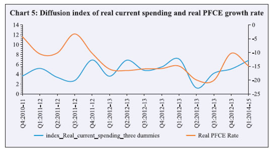 We also wanted to see whether the relationship between actual inflation and RPFCE growth matched our results or not. In other words, we examined whether CCS data were able to capture the relationship between actual inflation and consumer spending. Chart 6 shows the relationship between wholesale price inflation (WPI) rates, consumer price inflation (CPI) rates and RPFCE growth rates. CPI is negatively correlated with RPFCE growth rates. This exercise gives us additional confidence that the survey micro-data reflects the macroeconomic data, which is what it is intended to measure. Section VII
Summary and Conclusion The survey on consumer perceptions and expectations are of recent origin in India. This is the first study which empirically examines the effect of consumers’ inflation expectations on their spending behaviour using micro-survey data. It fulfils a major gap in our understanding of the evolution of consumer behaviour in an emerging market economy such as India. The evolving changes in economic structures associated with rapid economic growth and a developing socioeconomic stage provide an interesting opportunity to test some of the established works on consumer behaviour observed in advance societies such as the US and Japan. The cross-sectional nature of data provides necessary variance to test whether the relationship between inflation expectations and consumers’ spending change over time. Our results reveal that higher inflation expectations tend to result in greater current household spending and higher inflation expectations make consumers decrease their future spending. These results seem to be robust across various demographic and individual attributes of respondents and also over time. These results are useful inputs for monetary and macroeconomic policy for managing inflation from both supply and demand perspectives. Inflation management is important for sustained growth driven by consumption. The recent focus on managing inflation as a primary target for monetary policy is in line with the results of our study. There are various possible reasons for such behaviour observed among Indian consumers. Being a developing economy, Indian consumers’ major expenses are on basic sustenance needs like food, health and education. With a majority of the consumers being in the low/middle income group, there are future aspirations to be met through education (which has witnessed significant cost escalations). As a result, the persistent inflationary perceptions of the last few years have given a feeling of increased current spending and aspirations for reduced future spending. Moreover, Indian households are not known to save to take care of old age. These findings are in sync with results obtained by Ichiue and Nishiguchi (2013) for Japanese consumers. The commonality of consumer behaviour in Japan and India might be attributed to conservative spending traits and also the fact that both these economies witnessed very low ‘real interest rates’ until very recently. These results are, however, in contrast to the findings of Arnold et al. (2014), Bachmann et al. (2015) and Burke and Ozdagli (2013) wherein a negative insignificant relationship was observed. This difference could possibly be due to the different nature of data used. The findings of Bachmann et al. (2015) and Burke and Ozdagli (2013) were based on the US micro-survey data on ‘readiness to spend on large household durables’ while Arnold et al. (2014) used saving portfolio data. Going forward, similar studies with diverse consumers would help in improving our understanding of consumer behaviour. The inter-temporal results can be improved with a study of a panel of respondents. The present study covers one of the high inflation phases of the Indian economy and the robustness of results can be established covering various phases of an inflation cycle especially during low and stable inflation periods. With availability of long time-series data this issue can be revisited. Further studies on essential and discretionary spending will also help in improving our understanding of consumer behaviour.
References Ando, A. and F. Modigliani (1963), ‘The Life-Cycle Hypothesis of Saving: Aggregate Implications and Tests’, American Economic Review, 53: 55–84. Armantier, O., W. Bruin, G. Topa, W. Van der Klaauw and B. Zafar (2011), ‘Inflation expectations and behaviour: Do survey respondents act on their beliefs?’ Federal Reserve Bank of New York Staff reports 509. Arnold, E., L. Drager and U. Fritsche (2014), ‘Evaluating the link between consumers’ savings portfolio decisions, their inflation expectations and Economic news’, DEP (Socioeconomics) Discussion papers. Macroeconomics and Finance Series, Hamburg. Baba, N. (2000), ‘Exploring the Role of Money in Asset Pricing in Japan: Monetary Considerations and Stochastic Discount Factors’, Monetary and Economic Studies, 18(1): 159-198. Bachmann, R., T. O. Berg and E. R. Sims (2015), ‘Inflation Expectations and Readiness to Spend: Cross-Sectional Evidence’. American Economic Journal, EconomicPolicy, Vol 7 No.1 February 2015 1-35 An earlier version of this paper is circulated as NBER Working Paper No. 17958, March 2012. Bernanke, B. S. (1981), 'Permanent income, liquidity, and expenditure on automobiles: evidence from panel data’. NBER Working Paper No.756, September 1981. Burke, M. A. and A. Ozdagli (2013), ‘Household inflation expectations and consumer spending: Evidence from panel data’, Working paper 13-25 Federal Reserve Bank of Boston. Duesenberry, J.S. (1949), Income, Saving, and the Theory of Consumer Behaviour. Cambridge, Mass.: Harvard University Press. Eggertsson, Gauti B. and Michael Woodford (2003), ‘The Zero Bound on Interest Rates and Optimal Monetary Policy’, Brookings Papers on Economic Activity, 2:139–211. Friedman, M. (1957), A Theory of the Consumption Function. Princeton, NJ: Princeton University Press. Hamori, S. (1992), ‘Test of C-CAPM for Japan: 1980-1988’, Economics Letters, 38: 67-72. ______ (1996), ‘Consumption Growth and the Intertemporal Elasticity of Substitution: Some Evidence from Income Quintile Groups in Japan’, Applied Economics Letters, 3: 529-532. Ichiue, Hibiki and Shusaku Nishiguchi (2013), ‘Inflation Expectations and Consumer Spending at the Zero Bound: Micro Evidence’, Bank of Japan Working Paper No. 13-E-11, July. Available at: https://www.boj.or.jp/en/research/wps_rev/wps_2013/data/wp13e11.pdf. Juster, F. Thomas and Paul Wachtel (1972), ‘Inflation and the Consumer’, Brookings Papers on Economic Activity, Economic Studies Program, 3(1): 71-122. Krugman, P. R. (1998), ‘It’s Baaack: Japan’s Slump and the Return of the Liquidity Trap’, Brookings Papers on Economic Activity, 2: 137-205. Modigliani, F. and A. Ando 1957 – “Test of the Life Cycle Hypothesis of Saving”, Bulletin Oxford University Institute Stat. May issue 14, 99-124. Modigliani, F. and R.H. Brumberg, 1954 – “Utility Analysis and the Consumption Function – An Interpretation of Cross Section Data” in K.K. Kurihara ed. Post Keynesian Economics, New Brunswick, N.J. Rutgers University Press. Nakano, K. and M. Saito (1998), ‘Asset Pricing in Japan’, Journal of the Japanese and International Economies, 12: 151-166. Reserve Bank of India (2014-15), Handbook of Statistics on Indian Economy, Table 74, page 137. ______ (2014). ‘Consumer Confidence Survey - Q2:2013-14 to Q1:2014-15’, RBI Monthly Bulletin, September issue. Springer, W. L. (1977), ‘Consumer spending and the rate of inflation’, Review of Economics and Statistics, 59 (4): 299-306. Wiederholt, M. (2012), ‘Dispersed Inflation Expectations and the Zero Lower Bound’, Mimeo. Zeldes, S. P. (1989), ‘Consumption and Liquidity Constraints: An Empirical Investigation’, Journal of Political Economy, 97: 305-346.
Annexure II: Demographic Characteristics of Data | City | Percentage of respondents | | Bengaluru | 17.1 | | Chennai | 16.4 | | Hyderabad | 16.9 | | Kolkata | 16.7 | | Mumbai | 15.6 | | Delhi | 17.3 | | Total | 100.0 |
| Age-group | Percentage of respondents | | 22-60 | 91.8 | | 60 & above | 8.2 | | Total | 100.0 |
| Survey Round | Percentage of respondents | | Mar-11 | 6.9 | | Jun-11 | 6.6 | | Sep-11 | 6.5 | | Dec-11 | 6.9 | | Mar-12 | 7.0 | | Jun-12 | 6.8 | | Sep-12 | 6.7 | | Dec-12 | 6.8 | | Mar-13 | 7.0 | | Jun-13 | 6.8 | | Sep-13 | 6.7 | | Dec-13 | 6.9 | | Mar-14 | 5.2 | | Jun-14 | 6.5 | | Sep-14 | 6.8 | | Total | 100.0 |
| Gender | Percentage of respondents | | Male | 61.7 | | Female | 38.3 | | Total | 100.0 |
| Occupation | Percentage of respondents | | Employed | 58.6 | | Un-Employed | 41.4 | | Grand Total | 100.0 |
| Family Size | Percentage of respondents | | Up to 2 members | 7.9 | | 3 or 4 members | 52.6 | | 5 and more | 39.6 | | Grand Total | 100.0 |
Annexure III: Analysis taking Five Dummies for
Real Spending and Real Income Construction of dependent variable for model to examine the expected change in real spending Here we construct responses to an artificial question about the expected change in real spending in the next year by synthesizing the responses to the following two questions about price/inflation expectation (Question 14 in the CCS questionnaire) and expected change in nominal spending. First, associate each response to the two questions with a real number according to its contribution to nominal spending and prices to real spending. For Q9 on spending, responses ‘increase’; ‘neither increase nor decrease’; and ‘decrease’ are graded as +1, 0 and -1 respectively. Whereas for Q14 on expected prices, responses ‘will go up’ is graded as -1; ‘will remain almost unchanged’ as 0; and ‘will go down’ as +1. We define real spending as: Real spending = Expected nominal spending + expected inflation | | Q14 | | Increase | Same | Decrease | | Q9 | Increase | Same | Increase | Significantly increase | | Same | Decrease | Same | Increase | | Decrease | Significantly decrease | Decrease | Same | The responses to the synthesized real spending question are then defined as ‘increase significantly’ if the total sum is 2; ‘increase’ if total sum is 1; ‘remain the same’ if sum is 0; ‘decrease’ if total sum is -1; and ‘significantly decrease’ if total sum is -2. Theses synthesized responses of real spending are used as the dependent variable in the ordered probit model. Graded real numbers are used for determining the order of the nine combinations of nominal spending and price level, and the quantitative importance of each constructed response about expected real spending. Following a similar procedure, we construct an artificial dependent variable the ‘actual change in real spending’ by using the questions on changed consumption spending compared to one year ago and how perceptions on the overall prices of goods and services have changed compared to one year ago. The ordered probit model used in this case assumes that there is an unobserved variable for each observation i. The expected change in real spending can be modelled as: with threshold values α1, α2, α3 and α4. Using the maximum likelihood estimation procedure we estimate the ordered probit model as well as threshold values. The estimation results, using these constructed variables as dependent variables in the model are given in Tables A and B (in this Annexure) for economic and demographic controls respectively. | Table A: Estimation Results for Baseline Specifications | | Dependent variables: | Real spending one year from now (Model 1) | Real spending compared to one year ago (Model 2) | | Prices one year from now | | | | Increase | -1.339* (0.02) | 0.719* (0.02) | | Decrease | 1.142* (0.04) | -0.674* (0.04) | | Prices compared to one year ago | | | | Increase | | -1.943* (0.03) | | Decrease | | 1.500* (0.05) | | Economic conditions one year from now | | | | Improve | 0.138* (0.01) | 0.072* (0.01) | | Worsen | -0.099* (0.01) | 0.060* (0.02) | | Economic conditions compared to one year ago | | | | Improve | | 0.174* (0.02) | | Worsen | | 0.176* (0.01) | | Household circumstances compared to one year ago | | | | Better | | 0.248* (0.02) | | Worse | | 0.045* (0.01) | | Real income one year from now | | | | Significantly increase | 0.861* (0.05) | 1.103* (0.06) | | Increase | 0.510* (0.03) | 0.474* (0.03) | | Decrease | -0.343* (0.01) | -0.477* (0.01) | | Significantly decrease | -0.653* (0.02) | -0.727* (0.02) | | Real income compared to one year ago | | | | Significantly increase | | 1.081* (0.08) | | Increase | | 0.725* (0.04) | | Decrease | | -0.407* (0.02) | | Significantly decrease | | -0.692* (0.02) | | Employment scenario one year from now | | | | Improved | 0.124* (0.01) | 0.020 (0.01) | | Worsen | -0.130* (0.01) | -0.157* (0.01) | | Threshold | α1 = -2.998*
| α1 = -3.119* | | | (0.04) | (0.05) | | | α2 = -1.591* | α2 = -1.360* | | | (0.03) | (0.04) | | | α3 = 1.007* | α3 = 2.229* | | | (0.03) | (0.04) | | | α4 = 1.978* | α4 = 3.021* | | | (0.03) | (0.05) | | Number of observations : 75,573 | | Pseudo R2 : | 0.183 | 0.242 | Notes: The table reports the estimates of the results from the ordered probit baseline estimation.
‘* denote significance at the 1, per cent level. Standard errors are in parentheses. |
| Table B: Estimation Results for Baseline Specifications: Demographic Controls | | Dependent variables (with three dummies): | Real spending one year from now (Model 1) | Real spending compared to one year ago (Model 2) | | Independent Variables | Coefficients | Coefficients | | Gender | | | | Male | 0.021*** (0.01) | -0.044* (0.01) | | Age-group | | | | 22-60 | 0.021 (0.02) | -0.008 (0.02) | | Occupation | | | | Employed | -0.051* (0.01) | -0.030** (0.01) | | Annual income | | | | Up to Rs 1 lakh | -0.065* (0.01) | 0.009 (0.01) | | Family size | | | | Up to 2 members | -0.048* (0.02) | -0.130* (0.02) | | 3 or 4 members | 0.006 (0.01) | -0. 082* (0.01) | | City | | | | Bengaluru | 0.375* (0.01) | 0.099* (0.02) | | Chennai | -0.110* (0.02) | 0.335* (0.02) | | Hyderabad | 0.051* (0.01) | 0.392* (0.02) | | Kolkata | 0.269* (0.01) | 0.479* (0.02) | | Mumbai | 0.390* (0.02) | 0.152* (0.02) | | Notes: See the notes to Tables 1 and 2. The demographic controls include the dummy which takes unity for female respondents and 0 for males (sex); dummy which takes unity for respondents age less than or equal to 60 years and 0 otherwise; a dummy which takes unity for employed respondents and 0 otherwise. Moreover a dummy which take value 1 if respondent’s family size is less than or equal to 4 and 0 for family size greater than 4. |
Annexure IV: Analysis for Sub-sample taken from
Q2 2012-13 to Q3 2014-15 | Table C: Estimation Results for Baseline Specifications | | Dependent variables: | Real spending one year from now (Model 1) | Real spending compared to one year ago
(Model 2) | | Prices one year from now | | | | Increase | -1.617* (0.03) | 0.488* (0.03) | | Decrease | 1.592* (0.05) | -0.268* (0.05) | | Prices compared to one year ago | | | | Increase | | -2.120* (0.04) | | Decrease | | 1.478* (0.07) | | Economic conditions one year from now | | | | Improve | 0.036** (0.01) | 0.042* (0.02) | | Worsen | -0.130* (0.02) | -0.034* (0.02) | | Economic conditions compared to one year ago | | | | Improve | | 0.093* (0.02) | | Worsen | | 0.234* (0.02) | | Household circumstances one year from now | | | | Better | 0.061* (0.01) | 0.014 (0.02) | | Worse | -0.098* (0.02) | 0.009 (0.02) | | Household circumstances compared to one year ago | | | | Better | | 0.054* (0.02) | | Worse | | 0.207 * (0.02) | | Real income one year from now | | | | Significantly increase | -0.058 (0.06) | 0.518* (0.07) | | Increase | 0.084** (0.03) | 0.275* (0.04) | | Decrease | -0.132* (0.01) | -0.285* (0.02) | | Significantly decrease | -0.370* (0.02) | -0.614* (0.03) | | Real income compared to one year ago | | | | Significantly increase | | 0.926* (0.11) | | Increase | | 0.588* (0.05) | | Decrease | | -0.302* (0.02) | | Significantly decrease | | -0.375* (0.03) | | Employment Scenario one year from now | | | | Improved | 0.067* (0.01) | 0.054* (0.02) | | Worsen | -0.106* (0.02) | -0.164* (0.02) | | Employment Scenario compared to one year ago | | | | Improved | | 0.184* (0.02) | | Worsen | | 0.039*** (0.02) | | Threshold | α1 = -2.427*(0.07) | α1 =-3.006* (0.09) | | | α2 = -1.097* (0.06) | α2 =-1.132* (0.07) | | | α3 = 1.222* (0.06) | α3 =2.469* (0.07) | | | α4 = 2.186* (0.06) | α4 = 3.483* (0.07) | | Number of observations : 44,272 and 44,244 respectively | | Pseudo R2 | 0.168 | 0.210 | | Notes: The table reports the estimates of the results from the ordered probit baseline estimation.
*** ,** and * denote significance at the 10, 5 and 1 per cent levels respectively. Standard errors are in parentheses. |
| Table D: Estimation Results for Baseline Specifications | | Dependent variables: | Real spending one year from now (Model 1) | Real spending compared to one year ago (Model 2) | | Prices one year from now | | | | Increase | -1.621* (0.03) | 0.489* (0.03) | | Decrease | 1.205* (0.04) | -0.071 (0.04) | | Prices compared to one year ago | | | | Increase | | -2.193*(0.04) | | Decrease | | 0.907* (0.07) | | Economic conditions one year from now | | | | Improve | 0.082* (0.02) | 0.055* (0.02) | | Worsen | -0.024 (0.02) | -0.023 (0.02) | | Economic conditions compared to one year ago | | | | Improve | | 0.105* (0.02) | | Worsen | | 0.281* (0.02) | | Household circumstances one year from now | | | | Better | 0.077* (0.02) | 0.023 (0.02) | | Worse | -0.067* (0.02) | -0.007 (0.02) | | Household circumstances compared to one year ago | | | | Better | | 0.053** (0.02) | | Worse | | 0.234* (0.02) | | Real income one year from now | | | | Increase | 0.063 (0.03) | 0.272* (0.04) | | Decrease | -0.252* (0.02) | -0.337* (0.02) | | Real income compared to one year ago | | | | Increase | | 0.727* (0.05) | | Decrease | | -0.340* (0.02) | | Employment Scenario one year from now | | | | Improved | 0.128* (0.02) | 0.061* (0.02) | | Worsen | -0.062* (0.02) | -0.166 * (0.02) | | Employment Scenario compared to one year ago | | | | Improved | | 0.168* (0.02) | | Worsen | | 0.059* (0.02) | | Threshold | α1 = - 1.171* | α1 =-1.142* | | | (0.06) | (0.08) | | | α2 = 1.115* | α2 =2.477* | | | (0.06) | (0.08) | | Number of observations : 44,272 and 44,244 respectively | | Pseudo R2 | 0.208 | 0.241 | Notes: The table reports the estimates of the results from the ordered probit baseline estimation.
** and * denote significance at the , 5 and 1 per cent levels respectively. Standard errors are in parentheses. |
| Table E: Sub-sample Analysis Estimation Results for Baseline Specifications: Demographic Controls | | Dependent variables (with three dummies): | Real spending one year from now (Model 1) | Real spending compared with one year ago (Model 2) | | Independent variables | Coefficients | Coefficients | | Gender | | | | Male | 0.019 (0.02) | -0.096* (0.02) | | Age-group | | | | 22-30 | 0.018 (0.03) | -0.016 (0.03) | | 30-40 | 0.021 (0.03) | -0.018 (0.03) | | 40-60 | -0.002 (0.03) | 0.025 (0.03) | | Occupation | | | | Employed | -0.043 (0.03) | 0.007 (0.03) | | Self-employed/Business | -0.078* (0.03) | 0.004 (0.03) | | Housewife | -0.011 (0.03) | 0.018 (0.03) | | Daily worker | -0.055 (0.03) | -0.017 (0.04) | | Retired/pensioners | -0.058 (0.04) | -0.013 (0.04) | | Annual income | | | | Up to Rs 1 lakh | -0.101** (0.04) | -0.038 (0.04) | | 1-3 lakh | -0.107* (0.04) | -0.037 (0.04) | | 3-5 lakh | -0.006 (0.04) | -0.108** (0.05) | | Family size | | | | Up to 2 members | -0.020 (0.02) | -0.243* (0.03) | | 3 or 4 members | -0.003 (0.01) | -0. 119* (0.01) | | Educational qualification | | | | Up to primary | 0.044** (0.02) | -0.075* (0.02) | | Below graduate | 0.049* (0.02) | -0.033*** (0.02) | | City | | | | Bengaluru | 0.529* (0.02) | -0.031 (0.02) | | Chennai | 0.274* (0.02) | 0.527* (0.03) | | Hyderabad | 0.113* (0.02) | 0.510* (0.02) | | Kolkata | 0.379* (0.02) | 0.611* (0.02) | | Mumbai | 0.537* (0.02) | 0.273* (0.02) | | Notes: See the notes to Tables 1 and 2. The demographic controls includes the dummy which takes unity for female respondents and 0 for males (sex); dummy which take unity for respondents age less than or equal to 60 years and 0 otherwise; a dummy which take unity for employed respondents and 0 otherwise. Moreover a dummy which take value 1 is a respondent’s family size is less than or equal to 4 and 0 for family size greater than 4. |
| Table F: Estimation Results for Baseline Specifications: Demographic Controls | | Dependent variables (with five dummies): | Real spending one year from now (Model1) | Real spending compared to one year ago (Model 2) | | Independent variables | Coefficients | Coefficients | | Gender | | | | Male | 0.054* (0.02) | -0.114* (0.02) | | Age-group | | | | 22-30 | 0.001 (0.03) | -0.038 (0.03) | | 30-40 | 0.005 (0.03) | -0.044 (0.03) | | 40-60 | -0.014 (0.03) | 0.004 (0.03) | | Occupation | | | | Employed | -0.050*** (0.02) | 0.015 (0.03) | | Self- employed/business | -0.102* (0.02) | 0.020 (0.03) | | Housewife | -0.019 (0.03) | 0.012 (0.03) | | Daily worker | -0.079** (0.03) | 0.001 (0.03) | | Retired/pensioners | -0.075*** (0.03) | 0.005 (0.04) | | Annual income | | | | Up to Rs 1 lakh | -0.142* (0.04) | -0.067 (0.04) | | 1-3 lakh | -0.131* (0.03) | -0.051 (0.04) | | 3-5 lakh | -0.025 (0.04) | -0.077 (0.04) | | Family size | | | | Up to 2 members | -0.001 (0.02) | -0.241* (0.03) | | 3 or 4 members | 0.004 (0.01) | -0.114* (0.01) | | Educational qualification | | | | Up to primary | 0.048* (0.02) | 0.062* (0.02) | | Below graduate | 0.048* (0.01) | 0.030 (0.02) | | City | | | | Bengaluru | 0.409* (0.02) | 0.048*** (0.02) | | Chennai | 0.071* (0.02) | 0.545* (0.02) | | Hyderabad | -0.096* (0.02) | 0.518* (0.02) | | Kolkata | 0.395* (0.02) | 0.628* (0.02) | | Mumbai | 0.540* (0.02) | 0.320* (0.02) | | Notes: See the notes to Tables 1 and 2. The demographic controls includes the dummy which takes unity for female respondents and 0 for males (sex); dummy which take unity for respondents age less than or equal to 60 years and 0 otherwise; a dummy which take unity for employed respondents and 0 otherwise. Moreover a dummy which take value 1 if respondent’s family size is less than or equal to 4 and 0 for family size greater than 4. |
| Table G: Estimation Results for Baseline Specifications with Actual Nominal Spending (Rounds 4 to 20 data used for analysis): | | Dependent variables: | Nominal spending compared to one year ago | | Prices one year from now | | | Increase | 0.173* (0.02) | | Decrease | -0.009 (0.04) | Note: The table shows the estimated coefficient s on expected inflation for the specification using the responses about actual nominal spending growth as the dependent variable.
* denote significance at the 1 per cent level. Standard errors are in parentheses. |
| Table H: Estimation Results for Baseline Specifications with Actual Nominal Spending (Rounds 10 to 20 data used for analysis) | | Dependent variables: | Nominal spending compared to one year ago (real income as control variable) | | Prices one year from now | | | Increase | 0.444* (0.03) | | Decrease | -0.084*** (0.04) | Note: The table shows the estimated coefficients on expected inflation for the specification using the responses about actual nominal spending growth as the dependent variable.
***, and * denote significance at the 10 and 1 per cent levels, respectively. Standard errors are in parentheses. |
| Table I: Sub-sample Analysis by Individual Attributes (Rounds 10 to 20 data used for analysis) | | Dependent variables: | Real spending one year from now | Real spending compared to one year ago | | Prices one year from now: → | Increase | Decrease | Increase | Decrease | | Gender | | Female | -1.60* (0.03) | 1.537* (0.06) | 0.460* (0.04) | -0.301* (0.07) | | Male | -1.66* (0.04) | 1.692* (0.08) | 0.440* (0.05) | -0.156 (0.09) | | Age-group | | 22-30 | -1.642* (0.05) | 1.573* (0.09) | 0.382 * (0.05) | -0.264** (0.10) | | 30-40 | -1.605* (0.04) | 1.639* (0.08) | 0.428* (0.05) | -0.156 (0.09) | | 40-60 | -1.647* (0.05) | 1.507* (0.09) | 0.568* (0.05) | -0.366* (0.10) | | 60 and above | -1.573* (0.10) | 1.778* (0.16) | 0.446* (0.11) | -0.282 (0.18) | | Occupation | | Employed | -1.726* (0.05) | 1.577* (0.11) | 0.456* (0.06) | -0.167 (0.12) | | Self-employed/Business | -1.564* (0.05) | 1.585* (0.09) | 0.422* (0.06) | -0.368* (0.11) | | Housewife | -1.616* 0.05) | 1.703* (0.10) | 0.409* (0.06) | -0.273** (0.11) | | Daily worker | -1.545* (0.08) | 1.442* (0.14) | 0.597* (0.08) | -0.187 (0.16) | | Retired/pensioners | -1.655* (0.11) | 1.592* (0.19) | 0.537* (0.12) | -0.491** (0.22) | | Unemployed | -1.785* (0.10) | 1.685* (0.18) | 0.451* (0.10) | 0.118 (0.22) | | Annual income | | Up to Rs 1 lakh | -1.438* (0.04) | 1.539* (0.07) | 0.408* (0.04) | -0.065 (0.08) | | 1-3 lakh | -1.774* 0.04) | 1.665* (0.08) | 0.505* (0.04) | -0.466* (0.09) | | 3-5 lakh | -1.821* (0.09) | 1.331* (0.17) | 0.511* (0.09) | -0.293 (0.20) | | 5 lakhs and more | -1.628* (0.19) | 1.672* (0.36) | 0.353 (0.20) | -0.791 (0.42) | | Family size | | Up to 2 members | -1.521* (0.08) | 1.532* (0.16) | 0.481* (0.09) | -0.471** (0.18) | | 3 or 4 members | -1.657* (0.04) | 1.621* (0.07) | 0.516* (0.04) | -0.189** (0.08) | | 5 and more | -1.608* (0.04) | 1.617* (0.08) | 0.374* (0.05) | -0.284* (0.09) | | Educational qualification | | Up to primary | -1.680* (0.05) | 1.500* (0.08) | 0.447* (0.05) | -0.400* (0.09) | | Below graduate | -1.570* (0.04) | 1.741* (0.08) | 0.427* (0.04) | -0.188*** (0.09) | | Graduate and above | -1.681* (0.06) | 1.519* (0.10) | 0.559* (0.06) | -0.054 (0.12) | | City | | Bengaluru | -1.863* (0.07) | 2.033* (0.13) | 0.530* (0.07) | -0.004 (0.14) | | Chennai | -1.494* (0.07) | 1.389* (0.11) | 0.201** (0.08) | -0.083 (0.13) | | Hyderabad | -1.634* (0.06) | 1.468* (0.12) | 0.414* (0.07) | -0.260 (0.14) | | Kolkata | -1.942* (0.07) | 1.874* (0.13) | 0.497* (0.07) | -0.504* (0.15) | | Mumbai | -1.914* (0.08) | 1.749* (0.27) | 0.545* (0.08) | 0.417 (0.32) | | Delhi | -1.243* (0.06) | 1.483* (0.10) | 0.309* (0.07) | -0.040 (0.12) | Notes: The table reports the estimates coefficients on expected inflation for subsamples based on individuals’ attributes.
*, ** and *** denote significance at the 1, 5 and 10 per cent levels, respectively. Standard errors are in parentheses. |
|