Jai Chander* The government’s cash management operations are an integral part of its overall financial management. Apart from having direct implications in terms of financial costs to the government, cash management operations also interact with other policy domains such as debt management, monetary and liquidity management and financial markets. Some of the basic elements of an effective cash management framework include a single treasury account and accuracy in cash flow projections. The framework in India has seen major shifts towards use of market oriented instruments. A cash management strategy is often an integral part of debt management. An assessment of cash management in India indicates that volatility in cash balances was largely driven by revenues and borrowings from non-market sources, while expenditure was found to reduce the volatility. Against this background, the paper assesses the effectiveness of debt management strategy of the Government of India in managing volatility in its cash balances. Empirical evidence indicates that there have been effective modulations in the debt management strategy which have helped reducing volatility in cash balances. JEL Classification : C58, E61, E62 Keywords : Cash management, Debt management, Government Financial Statistics, GARCH Introduction A government’s financial management involves preparing the fiscal policy and budget, executing the budget and mobilising and using financial resources. Apart from accounting and auditing practices, cash management is an integral element of a government’s financial management which plays a critical role in the execution of the budget. The cash management function is performed with varying degrees of sophistication across countries depending on developments in areas of the control and forecasting mechanism of cash flows and the financial architecture of the country. The Government Financial Statistics (GFS) manual1 defines cash as notes, coins and deposits held on demand by government institutional units with a bank or another financial institution. ‘Cash equivalents’ are defined as highly liquid investments that are readily convertible to ‘cash on hand’. Depending on the level of advancements in a government’s financial management, cash is held in these two forms in varying proportions across countries. Cash management refers to managing both i.e., ‘cash on hand’ as well as ‘cash equivalents’. A government has a large number of inflows and outflows which may be identified in terms of government agencies associated with a particular cash flow and with debt and non-debt flows. Cash flows under certain heads such as salaries, interest payments and redemptions can be identified as different expenditure categories; advance tax receipts, indirect tax receipts, interest receipts, dividends, borrowings etc., can be identified as receipt categories. Most often, there are different agencies involved or associated with different categories of cash flows. The need for cash management by a government arises due to the need for timely availability of funds for spending agencies while minimising the cost of funds. Apart from this, a government’s cash management also enables containing aggregate spending, enhancing the efficiency of budget implementation and minimising the opportunity cost of resources (Lienert 2009). A government’s cash management and that of private business entities differs to a great extent as the government’s cash management has implications for the functions of the central bank, mainly liquidity management and to some extent monetary policy, particularly when the government decides to invest its surplus cash in market instruments. There is also a difference in the nature of cash flows of a government and that of a private business entity. A government has some regular inflows such as tax revenue which generally depends on macroeconomic factors outside the control of the government. A large part of a government’s spending responsibilities is independent of its inflows, at least in the short-term. Also, an equally large part of these responsibilities is committed and time-bound in nature reducing the manoeuvrability by government to fine-tune the outflows in sync with inflows. Against this background, the paper outlines the cash management framework of the Government of India and makes an assessment of effectiveness of the government debt management strategy in managing volatility in its cash balances. The rest of the paper is structured as follows: Section II presents basic elements of the cash management framework while Section III provides an interaction between cash management and other policy areas. Section IV discusses the cash management framework in India and Section V provides an assessment of cash management in terms of trends, sources of volatility and the role of debt management. Section VI gives concluding observations and policy implications. Section II
Basic Tenets of Effective Cash Management A government is an organisation of several units spread over a wide range of institutions/departments/agencies. While almost all the agencies are actively involved in varying degrees in government expenditure, revenue collection is often centralised in a few agencies/ departments. For effective cash management, it is essential that these inflows and outflows are aggregated on a daily basis and a system is developed to align inflows and outflows to the extent possible. By doing so, borrowings requirements for meeting temporary mismatches in inflows and outflows can be minimised. To meet these requirements, a cash management framework needs to have following essential features. Single Treasury Account The need for a single account where all government transactions are aggregated is probably the foremost requirement of effective cash management (Williams 2010). A government normally has multiple sub-accounts which belong to various agencies. These may be held with different banks. A single treasury account requires that transactions under all the sub-accounts are aggregated in a centralised single account, which is normally held with the central bank of the country. The centralised account is normally held in domestic currency and foreign currency is obtained from the central bank, whenever needed. However, a government may maintain a separate foreign currency sub-account within the centralised account. Cash Flow Projections Another basic requirement for effective cash management is reliable cash flow projections on a daily, weekly and monthly basis. The required periodicity and horizon of cash flow projections depend on the availability of cash management instruments and the development of the money market in the economy. Accuracy in cash flow projections enables effective investment of surplus cash and precision in borrowing schedule in case of a deficit. Availability of information about each spending agency and revenue collection department is crucial for precise cash flow projections. Cash flow projections can be done at each sub-account level and then the aggregated information can be used to arrive at the cash position of the central account. The central account section takes decisions on short-term borrowings and investment of surplus cash. In some countries like Australia each spending agency is also responsible for internal cash management. The end-of-day balances are swept into the treasury single account at the Reserve Bank of Australia. Thus, this system has a two-tier cash management: first at the level of spending agencies and second as a consolidated cash management system at the federal level. In France, on the other hand, the Agence France Tresor not only manages the central government’s cash balances but also of local governments and other public entities. Thus, cash flow projections differ in the two systems (Lienert 2009). Centralised cash flow projection depends more on statistical methods while decentralised cash flow projections mainly depend on non-statistical methods such as information available with spending agencies and revenue collection departments. Effective cash flow projections require a comprehensive framework whereby all the inflows and outflows are discretely identified. It may be useful to identify debt and non-debt cash flows separately as debt flows can also be used as an instrument of cash management. The cash management system requires a comprehensive enumeration and identification of each cash flow. The budget provides revenue and expenditure estimates for the full year. Daily, weekly or quarterly cash flow projections need to be consistent with the overall revenue and expenditure estimates provided in the budget. Sometimes the revenue and expenditure estimates provided in the budget may not be a simple aggregation of daily cash flows as daily cash flows may include some extra-budgetary transactions. These extra-budgetary items, however, have an impact on a government’s cash balance position and may sometimes require the government to borrow short-term cash.2 Cash flow projections, thus, require the identification of all such transactions and then explicitly accounting for them so that consistency between budgetary revenue and expenditure is maintained. Apart from facilitating cash management, such consistency also enables a government to take corrective measures during the course of the year if it is realised that there could be deviations from budgetary revenue and expenditure targets. Section III
Cash Management: Interaction with other Policy Domains Cash management is an integral part of debt management which allows a government to raise its long-term borrowings in a planned manner; this also facilitates efficient management of investors. Cash flows of financial institutions are normally distributed across the year. Hence, an evenly distributed market borrowings programme across the year, which is broadly in sync with the cash inflows of investors, is likely to be cost effective for a government. Though such a programme may promote the objective of cost minimisation in the medium and long-term, it may not be consistent with intra-year cash flow. An efficient cash management system enables a government to plan out its long-term market borrowings programme in a cost effective manner and use the cash management framework to manage intra-year cash deficit/surplus. A government’s cash management also interacts with the financial markets, particularly the money market and with liquidity management by the central bank (Pessoa and Williams 2012). A government’s surplus cash is invariably kept with the central bank. Thus, an increase in a government’s surplus cash with the central bank leads to an equivalent shortage of liquidity in the system. The central bank, therefore, needs to monitor the cash flows of the government while fine-tuning its liquidity management operations. Government’s decision regarding its dependence on central bank or recourse to market for cash requirements or for investing surplus cash will have direct implications for the money market. The impact of a government’s cash management operations on the market can be significant because government transactions generally involve relatively large amounts as compared to other market participants. In a market determined exchange rate, government’s cash management operations may also interact with the foreign exchange market by influencing short-term interest rates. Globally, capital accounts have been increasingly liberalised to allow for capital flows in equity as well as debt markets. Near zero rate policies followed in advanced economies in the post-crisis period encouraged even more capital inflows in debt markets in emerging market economies. While this trend enabled lowering borrowing costs in these economies, their capital accounts have become more vulnerable and sensitive to interest rate movements. Ahmed and Zlate (2013) conclude that while the growth differential was the major factor in determining capital inflows to emerging market economies before the crisis, policy rate differential emerged as an equally important factor influencing such flows post crisis. Short-term interest rates in most countries depend on policy rates which are decided by the respective central banks. The usual practice is to set a band for policy rates and the provision of liquidity by the central banks at these rates ensures that overnight rates remain within the policy rate band. Overnight rates also play a crucial role in shaping short-term interest rates on the extent to which market players can roll over their borrowings from the central bank. Government’s cash management operations may not influence the short-term rates significantly if the central bank provides/absorbs adequate or unlimited liquidity to/from the market. In case the central bank decides to provide/absorb liquidity within limits, a government’s cash management may significantly influence short-term interest rates in the economy. This may have significant implications for capital flows and the exchange rate, particularly when the short-term debt market is open to foreign capital. Section IV
The Cash Management Framework in India This section provides a description of central government’s cash flows with a view to building an analytical framework. The Government of India’s cash management stems from the Union Budget which sets out the magnitude of cash transactions for the next year in terms of revenue and expenditure. The budget also provides estimates of the net amount to be borrowed under different sources of financing to fill the gap between revenue and expenditure represented by gross fiscal deficit (GFD). Apart from GFD, cash flows may witness deficit/surplus on account of some transactions which may not be part of the GFD calculations. Receipts and expenditures of some public enterprises are taken into account on a net basis in calculating GFD, while for cash management purposes gross receipts and expenditures are the relevant variables. Similarly, repayments of debt are kept out of GFD’s calculation while for cash management purposes they are often crucial parameters. Receipts The receipts of the government consist of tax revenue, non-tax revenue, disinvestment proceeds and borrowings. Tax revenue mainly comprises of direct and indirect taxes. Cash flows of direct taxes depend on the stipulated rules for making tax payments. Barring the tax deducted at source which is credited to the government account on a monthly basis, direct tax payments are made on a quarterly basis in June, September, December and March. The final payments are made at the end of the financial year, usually during the last week of the year. Regarding indirect taxes, payments by taxpayers are made on a monthly basis. The Central Excise Rules 2002 stipulate, ‘the duty on the goods removed from the factory or the warehouse during a month shall be paid by the 6th day of the following month, if the duty is paid electronically through internet banking and by the 5th day of the following month, in any other case’ (CBEC Rules 2002). In the case of goods removed during March, the duty is to be paid by the 31st day of March. Regarding service tax, the Point of Taxation Rules 2011 stipulate that the date of payment shall be the earlier of the dates on which the payment is entered in the books of accounts or is credited to the bank account of the person liable to pay tax. Customs duties are normally paid at the time that goods are imported in the country, which may not follow a predictable pattern. The government’s non-tax revenues are in the form of interest receipts, dividends and profits of public sector enterprises and user charges. Disinvestment by the government is planned in view of market conditions, hence cash flows related to these proceeds may be predictable only to the extent that the disinvestment plan is known. The government’s borrowings may be categorised into market and non-market borrowings. Non-market borrowings include receipts under the public account such as small savings and provident fund, external assistance, investment in 14-day intermediate treasury bills by state governments and other items. Market borrowings for cash management purposes can be defined to include dated securities, treasury bills and cash management bills. Market borrowings, particularly treasury bills and cash management bills, are planned in view of the cash flow pattern of the government. Non-market borrowings may not follow a predictable pattern and may influence cash flows significantly. Apart from this, the government also receives ways and means advances from the Reserve Bank, which are basically provided to manage temporary mismatches in cash flows. Disbursements Disbursements of the government consist of expenditures under various heads. For cash management purposes, it is useful to classify these expenditures on the basis of predictability of cash flows. Interest payments and redemptions of debt are usually known in advance and therefore it is easy to predict the timeline for these transactions. The government’s expenditure on payment of salaries and pensions follows a monthly pattern. The government also makes payments in terms of transfers to state governments as share in central taxes and grants-in-aid, which are made on a monthly basis. Apart from these, there are other capital and revenue expenditures which necessitate the development of a framework for making projections for cash management purpose. Exchange of information and coordination with spending line-ministries is crucial while making projections on cash flows with respect to these expenditures. Institutional framework for cash management The basic framework for the Government of India’s cash management is encapsulated in the Indian Constitution and the Reserve Bank of India Act 1934. Article 283(1) and (2) of the Indian Constitution prescribe that the central and state governments may make rules for the receipt, custody and disbursement of all the amounts accruing to or held in its consolidated or contingency funds or in its public account. Sections 20 and 21 of the Reserve Bank of India (RBI) Act 1934 provide that the central government shall entrust the Reserve Bank with all its money, remittances, exchange and banking transactions in India and the management of its public debt, and shall also deposit all its cash balances with the Reserve Bank free of interest. The Reserve Bank may, by agreement with any state government, take over similar functions on behalf of that government under Section 21A of the RBI Act. Accordingly, the Reserve Bank is the debt manager for all the 29 state governments and the union territory of Puducherry as also a banker to them except the Government of Sikkim in terms of their agreements with the Reserve Bank (RBI 2015). Thus, the Reserve Bank acts as banker to the Government of India under RBI Act 1934. Government transactions are undertaken directly by the Reserve Bank as well as through agency banks. All transactions are reported to the Reserve Bank by agency banks. The cash position is reflected in the single aggregated account which may be called a single treasury account. The government is required to maintain a minimum balance of ₹10 crore in its account on a daily basis and ₹100 crore on Fridays (Reddy 2002). Instruments to replenish shortfalls from the minimum cash balance have changed over time. Prior to 1997, issuance of ad hoc treasury bills was the primary instrument for making up the shortfall in minimum cash requirements which was initially fixed at ₹4 crore ( ₹50 crore on Fridays). To adhere to this administrative arrangement, it was agreed that the Reserve Bank would replenish the government’s cash balances by creating ad hoc treasury bills in favour of the Reserve Bank. The ad hoc treasury bills, which were meant to be temporary instruments, gained a permanent as well as a cumulative character as these were converted to dated securities periodically. Indeed, it became an attractive source of financing government expenditure since it was available at an interest rate pegged at 4.6 per cent per annum since 1974 (Reddy 1997). The system of ad hoc treasury bills implied automatic issuance of treasury bills by the government to Reserve Bank. As the ad hoc treasury bills were periodically converted into dated securities, this practice led to rapid monetary expansion, as fiscal deficit became a prominent and regular feature of the government’s budget. Accordingly, the need was felt to stop the system of ad hoc treasury bills. With a mutual agreement between the Reserve Bank and the Government of India, a limit was placed on issuance of ad hoc treasury bills which remained operative during 1994-95 to 1996-97. In 1997, the system of issuing ad hoc treasury bills was discontinued and a system of ways and means advances (WMA) was introduced with an agreement between the government and the Reserve Bank. An important step in the direction of cash management was the setting up of a Monitoring Group on Cash and Debt Management to decide on the implementation of the borrowing programme based on proposals made by the Reserve Bank. This is a standing committee of officials from the Ministry of Finance (MoF), Government of India and the Reserve Bank. While this represents a formal working relationship between MoF and the Reserve Bank, it is further complemented by regular discussions between the ministry and the Reserve Bank (GoI 2008; Khan 2014). WMA’s objective was to accommodate temporary mismatches in the government’s receipts and payments. Its limits are periodically revised in consultation with the government. It was agreed by the government and the Reserve Bank that when 75 per cent of the WMA limits are utilised, the Reserve Bank would trigger a fresh floatation of government securities. Though the WMA system has transformed the paradigm of fiscal-monetary interaction in India, it remains a matter of debate whether the new system has imparted the sensitivity and hard budget constraints that were expected (Reddy 2000). Moreover, it has been argued that excessive recourse to WMA/overdrafts by the government creates primary liquidity in the system. Realising the increased volumes of government transactions and the adverse impact of taking recourse to WMA/overdraft in terms of money creation, the government in consultation with RBI introduced cash management bills (CMBs) in 2010-11. The first auction of CMBs was held on May 11, 2010 for ₹6,000 crore. CMBs are discounted instruments like treasury bills but of a non-standard maturity of less than 91 days. These instruments have not only emerged as effective tools to reduce taking recourse to WMA but have also enabled the government to smoothen its cash balances. Dated securities and treasury bills are issued as per the pre-announced calendar, preparation of which also takes into account the government’s cash flows. Particularly, treasury bills of shorter maturity of 91 days can be effectively used for cash management purposes. The government and Reserve Bank are also developing instruments of buyback/switch. The response to the initial buyback offer in 2003 was muted; however, later offers in 2010-11 and 2013-14 were well received. In summary, the instruments which are employed for cash management include CMBs, treasury bills, scheduling of borrowings through dated securities and buyback/switch of debt. The Reserve Bank’s WMA/OD facility is used to meet residual temporary mismatches in receipts and expenditures. From December 16, 2014, onwards, the government’s cash balances held with the Reserve Bank are being reckoned for auction through variable rate repo as part of the Reserve Bank’s revised liquidity management framework (RBI 2015). Section V
Assessment of Cash Management in India Apart from the annual data provided in the Union Budget, data on the central government’s fiscal operations are available on a monthly basis as brought out by the Controller General of Accounts (CGA), Government of India. It is pertinent to mention here that there are differences between fiscal balance and cash balance. The two may move in the same direction but can differ in magnitude to a large extent. The differences are mainly due to the fact that cash balances capture the impact of below-the-line items. For instance, redemption of debt and public account receipts/disbursements affect the cash balance but not the fiscal balance. CGA provides data on increase/decrease in cash balance, investment/disinvestment of surplus cash and WMA. The overall cash position of the government is essentially the sum of all these components. For this study, however, cash balances are defined as position before investment/disinvestment/WMA, which is a function of the government’s receipts and disbursements. Data on cash balances as well as other fiscal variables for this section are obtained from CGA, while data on market borrowings are sourced from the Handbook of Statistics on Indian Economy, Reserve Bank of India and the Handbook of Statistics on Central Government Debt, Government of India. The data are for April 1999 to March 2015 as consistent monthly data were available from April 1999. As discussed earlier, the major fiscal variables which determine cash balance variations may broadly be classified as receipts, expenditures and borrowings. For analytical purpose, receipts have been grouped as revenue receipts (RR) which consist of net tax revenue (NTR) and non-tax revenue (non-tax). Apart from this, two more categories of receipts are considered for analysis -- gross tax revenue (GTR), that is, total tax revenue including states’ share and non-debt receipts (NDR) which include RR and other non-debt capital receipts such as disinvestments and recovery of loans. Major disbursements or total expenditure (TE) can be categorised as revenue expenditure (RE) and capital expenditure (CE). Further, receipts from borrowings are categorised as market borrowings (MB) including dated securities, treasury bills and CMBs; public account and external borrowings (PActExt) and others which mainly include states’ investments in 14-day treasury bills. Based on this classification, monthly cash balances of the government may be defined as: Casbal = NDR – TE + MB + PActExt + others It may be noted that cash balance is different from fiscal balance which may be defined as: Fiscal deficit = TE – NDR Trends in Cash Balances and Fiscal Variables As discussed earlier, data on cash balances (casbal) and other fiscal variables of the central government are available on a monthly basis, wherein daily variations in cash balances are likely to be averaged out. A simple plot of monthly variations in cash balances reveals two prominent features. First, there is a significant increase in monthly variations in cash balances inter alia reflecting inflationary impact as cash balances get recorded in nominal values. Second, the large variability in cash balances is against expectations of a smoother series due to averaging out of daily variations in the monthly data (Chart 1). Cash balances net of market borrowings including treasury bills (casnetb) show even greater variability. For instance, the range of cash balances net of borrowings at ₹(-)1,44,536-1,12,331 crore was wider than the range of ₹(-)1,03,986-87,133 crore for cash balances, indicating the impact of market borrowings in terms of reduction in the volatility of the cash position.  Notwithstanding a sharp rise in monthly cash balances, the annual average cash balance (Average) remained broadly unchanged over time with monthly variations getting averaged out over the year (Chart 2). The annual average cash balances net of borrowings (AverageNB) showed increasing deficit over the years in line with a nominal increase in gross fiscal deficit. Intra-year standard deviations (StDev) of overall cash balances are generally less than that of the cash balances adjusted for market borrowings (StDevNB) reflecting the daily variations getting evened out over the month. Nevertheless, the difference between the two standard deviations is seen to be increasing in recent years reflecting an improvement in the effectiveness of the market borrowing strategy in reducing volatility in the government’s cash balances. A significant drop in variability in cash balances AverageNB since 2011-12 can partly be attributed to the government taking large recourse to issuance of CMBs which were introduced in 2010-11. Apart from CMBs, market borrowings through dated securities, treasury bills and buyback/switches are also scheduled taking into account the cash flows of the government. 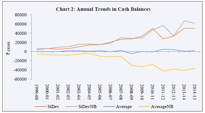 With a view to tracing the sources of variations in cash balances, it is useful to begin with the simple correlation of fiscal variables with cash balances. If market borrowings are scheduled to smoothen cash balances, it makes sense to examine the correlation of fiscal variables with cash balances net of market borrowings (casnetb) as well (Chart 3). It is evident from the pattern of correlations that receipts are strongly related with cash balances as compared to expenditure. Within receipts, non-tax revenue appears to have a relatively lesser significance while tax revenue and non-debt capital receipts, which are constituents of NDR, appear to be relatively stronger factors influencing cash balances.3 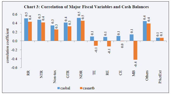 As expected, expenditure shows a negative correlation with cash balances (net of market borrowings) but the correlation magnitude is lower compared to that of revenue. A higher and negative correlation of market borrowings, which are not part of casnetb, indicates that the market borrowings are scheduled keeping in view the cash position in such a way that the borrowings are increased when cash balances decline. Another variable which deserve some discussion is ‘others’, which includes states’ investments in 14-day intermediate treasury bills. A relatively greater association of ‘others’ with cash balances indicates the role of states’ finances in the central government’s cash balances. The overall expenditure of the government has not only shown a smoother intra-year pattern, the degree of volatility too has declined over the years barring 2014-15 which showed an upturn in volatility (Chart 4). The central government’s NTR showed a consistently higher intra-year volatility primarily reflecting the impact of quarterly tax inflows and tax refunds at the beginning of each year. Non-tax revenue showed some spikes in intra-year volatility in 2007-08 and 2010-11. The former was due to negative non-tax revenues in September 2007 and increased volatility in 2010-11 reflects the impact of telecom receipts arising from spectrum auctions. Sources of Volatility in Cash Balances To further analyse the sources of volatility in government cash balances, a more formal measurement of volatility using the GARCH model was attempted. The GARCH model is suitable for modelling volatility in monthly fiscal variables which tend to show a time varying volatility. The analysis involved two steps. In the first step, volatility of each variable was estimated using the GARCH (1, 1) model. While doing so, usual diagnostics for the presence of ARCH effects and stationarity of variables were undertaken before generating the residual series from the model. The second step was estimating the coefficients using the least square method and also conducting pair-wise Granger causality tests for a relationship between volatility in fiscal variables and cash balances. The conclusions are drawn on the basis of the results and theoretical background of the relationships between the variables. Two main sets of equations were estimated for analysis. One for the government’s cash balances in terms of monthly variations in the cash balance position of the government and second for cash balances net of borrowings which are closer to monthly fiscal deficit. Regression equation (1) explains volatility in cash balances (vcasbal) in terms of volatility in major fiscal variables viz., non-debt receipts (vndr), total expenditure (vte), net market borrowings (vnetdebt) and net receipts from other financing items (vothersall). As expected, volatility in non-debt receipts contributed positively to volatility in cash balances while a negative coefficient of expenditure indicated a possible expenditure modulation by the government in view of its cash balance position. The equation also indicates that market borrowings contributed positively to the volatility in cash balances. There was, however, a need for testing for Granger causality to further confirm the direction of causality. Theoretically, one can expect a reasonable level of discretionary elements in expenditures and borrowings and therefore these instruments can also be used as cash management instruments.  Coefficients of regression equation for volatility in cash balances net of market borrowings (vcasnetb), reported in equation (2), are in line with estimates in equation (1). Before measuring the volatility, net receipts from market borrowings were netted out of cash balances so that the cash balance remained an outcome of revenue, expenditure and other financing items. Other financing items include state governments’ investments in 14-day intermediate treasury bills of the central government and are often considered to be a major source of volatility in the central government’s cash balances. Volatility in Cash Balances: Causes and Effects Regression estimates in equation (1) indicate a negative association between expenditure and cash balance volatility and pair-wise Granger causality test, reported in Table 1, indicates that causality runs from volatility in expenditure to volatility in cash balances. This is clear evidence of the government increasing its expenditure when cash balances are high and reducing it when cash balances decline in such a manner that higher volatility in expenditure leads to lower volatility in cash balances. In fact, the results imply the possibility that the government increases or reduces its expenditure in anticipation of its cash balance position so that it is the expenditure which influences volatility in cash balances and not the other way round. Other financing items (vothersall) were found to affect cash balances with 2 lags while other way causation was not statistically significant. Combining these results with the coefficient in regression equation (1) leads us to conclude that volatility in other financing items contributed positively to volatility in the government’s cash balances. A pair-wise causality test between net market borrowings and cash balances indicates that volatility in cash balances affects volatility in market borrowings implying that the government’s cash flow pattern influences its debt management strategy. | Table 1: Pair-wise Granger Causality Tests | | Null Hypothesis: | Obs | F-Statistic | Prob. | | With one lag | | VTE does not Granger Cause VCASBAL | 190 | 11.3893 | 0.0009 | | VCASBAL does not Granger Cause VTE | 0.26368 | 0.6082 | | VOTHERSALL does not Granger Cause VCASBAL | 190 | 0.11585 | 0.7340 | | VCASBAL does not Granger Cause VOTHERSALL | 1.17122 | 0.2805 | | VNETDEBT does not Granger Cause VCASBAL | 190 | 4.76045 | 0.0304 | | VCASBAL does not Granger Cause VNETDEBT | 25.8097 | 9.E-07 | | With two lags | | VTE does not Granger Cause VCASBAL | 189 | 13.6477 | 3.E-06 | | VCASBAL does not Granger Cause VTE | 0.55543 | 0.5748 | | VOTHERSALL does not Granger Cause VCASBAL | 189 | 6.06485 | 0.0028 | | VCASBAL does not Granger Cause VOTHERSALL | 2.69971 | 0.0699 | | VNETDEBT does not Granger Cause VCASBAL | 189 | 1.61814 | 0.2011 | | VCASBAL does not Granger Cause VNETDEBT | 18.8885 | 3.E-08 | | Note: Rejects null when probability value is less than 0.05 | Interaction of Cash and Debt Management One of the essential features of an effective debt management strategy is responding to cash requirements of the government and effectively meeting its requirements in a market oriented manner. An assessment of the effectiveness of debt management in India from this perspective is attempted with the help of data on monthly cash balances (net of borrowings) and net debt receipts. Suitable transformations in the data were undertaken to arrive at monthly deviations from annual averages for the respective variables in following manner: Xit = Xi – avgXt ……….. (i represents month and t represents year) The resulting variable (Xit) was then stacked for all the years. An effective debt management strategy requires increasing borrowings in those months when deviations in cash balances from annual average are negative, that is, the cash balance for the month is less than the average for the year. A simple regression equation estimates for cash balances (net of borrowings) and net debt receipts using this methodology are given in equations (3) and (4). It is evident from the coefficients that the response of market borrowings to a decline in cash balances was statistically significant and positive, that is, there was an increase in market borrowings for those months when cash balances were less than the annual average. Furthermore, the regression estimates were better when estimated for the shorter sample period from 2011 to 2015 (equations 5 and 6) as reflected in terms of improvement in adj.R2 and also the significance level of coefficients. This indicates a more active use of debt management strategy both through dated securities and treasury bills in recent years. (Sample period from 2011 to 2015) The pair-wise Granger causality test (Table 2), confirms that a lower than average cash balance (net of borrowings) triggered an increase in borrowings through dated securities and treasury bills. Even though the unexplained variation remains relatively large in the equations, the absence of other way round causality indicates the effectiveness of the debt management policy, insofar as cash management is concerned. | Table 2: Pair-wise Granger Causality Tests | | Null Hypothesis: | Obs | F-Statistic | Prob. | | NETBILLS1 does not Granger Cause CASHNET1 | 190 | 1.89843 | 0.1527 | | CASHNET1 does not Granger Cause NETBILLS1 | | 7.34382 | 0.0009 | | NETDEBT1 does not Granger Cause CASHNET1 | 190 | 2.78022 | 0.0646 | | CASHNET1 does not Granger Cause NETDEBT1 | | 11.1310 | 3.E-05 | | NETDEBT1 does not Granger Cause NETBILLS1 | 190 | 0.82987 | 0.4377 | | NETBILLS1 does not Granger Cause NETDEBT1 | | 0.28024 | 0.7559 | Section VI
Conclusion The government’s cash balances are different from fiscal deficit and have different monetary and liquidity management implications. Apart from revenues and expenditures, cash balances are also influenced by borrowings through various means. Empirical evidence indicates that volatility in the government’s cash balances was largely driven by revenues and borrowings from non-market sources, while the expenditure pattern was found to bring down volatility in cash balances. An effective debt management strategy should, inter alia, take into account the cash position of the government and modulate the borrowing schedule so that its cash requirements are met and at the same time excessive accumulation of cash balances is avoided. Findings in this paper indicate evidence of effective modulations in the debt management strategy so as to reduce volatility in cash balances. Furthermore, the effectiveness of the debt management strategy was found to have improved in recent years. It is submitted that weekly data might to be more useful in bringing out these results more conclusively, and the availability of this remains a limitation of this paper. From the policy perspective, the findings of the paper indicate that debt management can be effectively used to smoothen out volatility in the government’s cash balances. Improvements in the effectiveness of the debt management strategy in recent years underline the importance of the active use of short-term debt instruments such as treasury bills and cash management bills in smoothly managing cash flows. Since the use of such instruments will not be without costs, there may also be merit in leveraging fiscal policy instruments for cash management such as aligning expenditure with revenue flows or putting in place a mechanism for more smooth revenue flows. Another item, financing from non-market sources, was also found to be a source of volatility in the government’s cash balances which may be examined to see if there is some scope of reducing its variations.
References ADB (1999), ‘Managing Government Expenditure’ April. Available at: http://www.adb.org/publications/managing-government-expenditure Ahmed, Shaghil and Andrei Zlate (2013), ‘Capital Flows to Emerging Market Economies: A Brave New World?’ International Finance Discussion Papers Number 1081; Federal Reserve System; June. Available at: www.federalreserve.gov/pubs/ifdp/2013/1081/ifdp1081.pdf CBEC Rules (2002), Available at: http://www.cbec.gov.in/excise/cxrules/cx-rules-2002.htm GoI (2008), ‘Establishing a National Treasury Management Agency’; Report of the Internal Working Group on Debt Management; Department of Economic Affairs; Ministry of Finance; Government of India (GoI), New Delhi. Available at: http://www.finmin.nic.in/reports/report_internal_working_group_on_debt_management.pdf Khan, H.R. (2014), ‘Public Debt Management: Reflections on Strategy & Structure’; based on the keynote address at the 9th Annual International Conference on ‘Public Policy & Management: Debt Management’, at the Indian Institute of Management, Bengaluru on August 11, 2014. Available at: https://www.rbi.org.in/scripts/BS_SpeechesView.aspx?Id=909 Lienert, Ian (2009), ‘Modernizing Cash Management, IMF Technical Notes and Manuals’. Available at: http://www.imf.org/external/pubs/ft/tnm/2009/tnm0903.pdf Pessoa, Mario and Mike Williams (2012), ‘Government Cash Management: Relationship between the Treasury and the Central Bank’; IMF Technical Notes and Manuals; November. Available at: https://www.imf.org/external/pubs/ft/tnm/2012/tnm1202.pdf RBI (2015), Annual Report 2014-15. Mumbai: The Reserve Bank of India. Reddy, Y.V (1997), ‘The new directions being embarked upon in India with respect to the national budget and the Reserve Bank of India’, Address at the Administrative Staff College in Hyderabad. Available at: http://www.bis.org/review/r970321b.pdf ------ (2000), ‘Fiscal and Monetary Policy Interface: Recent Developments in India’; Speech at Workshop on Budgeting and Financial Management in the Public Sector, John F. Kennedy School of Government, Harvard University, Cambridge, Massachusetts, USA on August 10. ----- (2002), ‘Economic reforms and evolving role of RBI as banker to the governments’; Address at the Conference of the Silver Jubilee Celebrations of the Indian Civil Accounts Organization, New Delhi, 3 April. Available at: http://www.bis.org/review/r020405c.pdf Williams, Mike (2010), ‘Government Cash Management: Its Interaction with Other Financial Policies’, IMF Technical Notes and Manuals; IMF, July. Available at: https://www.imf.org/external/pubs/ft/tnm/2010/tnm1013.pdf
|