Sangita Misra and Pushpa Trivedi*

The 2008 global financial crisis reinforced the Keynesian argument that fiscal policy can be an important tool for influencing growth inflation dynamics. However, recognizing that using the headline fiscal balance to assess fiscal stance may incentivise bad policies in good times and penalize good policies in bad times, disentangling the overall fiscal balance into cyclical and structural components has been the current focus in literature. The last two decades have seen a large number of countries, both advanced and emerging, using this concept in their official functioning to enhance fiscal transparency. Of late, the G20 countries are deliberating on using structural fiscal balance as one of the supporting structural indicators to assess member countries’ fiscal reforms along with other indicators. Enlisting the various institutional approaches that have evolved over the years in the global arena to compute structural fiscal balances, this paper computes structural balances for India using the OECD and ECB approaches. The study finds that the automatic impact of output cycles and tax base cycles (also called output composition in the literature) on fiscal policy could be to the extent of 0.6-0.7 per cent and 0.2-0.4 per cent of GDP, respectively depending on output gap estimates using a range of empirically estimated elasticities and taking into account the one-offs. Hence, structural fiscal balances for India, on an average, could be at least about 0.8 percentage points more or less than what is actually observed.

JEL Classification : E62, E32, H62
Keywords : Fiscal Policy, Business Cycles, Structural Fiscal Deficit, Tax Base

Introduction

While the global financial crisis revived interest in the role of a discretionary fiscal policy as a macroeconomic stabilisation instrument, the fiscal/debt problems post the crisis have enhanced the need for using this tool more judiciously and appropriately and enhancing fiscal transparency. One step in this direction has been assessing the fiscal policy not in terms of headline fiscal balance, but in cyclically adjusted terms, that is, by removing the impact of business cycles on fiscal variables given the pivotal role that business cycles can play in fiscal policy. An augmentation of cyclically adjusted balances are structural balances which adjust for other non-structural elements like temporary financial sector or asset price movements, tax base cycles and other one-off revenues/expenditures. While on the one hand, such a concept allows the accommodation of external shocks beyond the control of the authorities, on the other hand it acts as a check on authorities not to overspend during good times (upturns) and conserve for bad times (downturns). Thus, while it helps reduce the procyclicality of fiscal policy, it can also be used as a good buffer.

While the concept of Structural Fiscal Balance (SFB) is not new to the literature, it has attracted global attention significantly in the last few years so as to assess nations’ fiscal policy that could be deemed independent of cycles of output, asset and commodity prices. International institutions like the International Monetary Fund (IMF) and the Organisation for Economic Cooperation and Development (OECD) have conducted extensive research in this area and are encouraging economies to adopt and publish fiscal stance after due adjustments for business cycle impact (Bornhost et al. 2011; Fedelino et al. 2009; Girouard and Andre 2005). Many developed countries including the EU and some emerging economies have been using this concept of SFB in their policy analysis. Some countries have gone one step ahead and adopted this concept in their fiscal rules. Setting up fiscal rules in terms of cyclically adjusted/structural balances is considered better than general balances as targeting the cyclically adjusted balance (CAB) tends to improve fiscal transparency and enhance the stabilizing properties of the rule.

In India, fiscal stance is generally analysed in terms of headline fiscal balance. Research in India in the area of cyclically adjusted fiscal policy is rather limited and the computation of structural fiscal balances is practically non-existent.¹ For a developing economy like India, a counter-cyclical fiscal policy could be an important stimulating tool as witnessed during the crisis. However, controlling fiscal deficit at a reasonable level is important both from the debt sustainability and inflation perspectives (RBI 2013a). Thus, fiscal policy as a tool needs to be used prudently and judiciously. It is in this context that the concept of SFB becomes relevant. In fact the 2000s, and more particularly the post global financial crisis period (which was characterised by large scale use of a counter-cyclical fiscal policy), has seen a surge in literature on this for emerging markets which at times has culminated in changes in official policies as well. The government of India in its 2015-16 Budget emphasised the need to look into cyclical considerations in analysing the budget and in the 2016-17 Budget, the need to revisit the overall medium term fiscal plan as well as the Fiscal Responsibility and Budget Management (FRBM) Act was emphasised. At the global level also there is peer pressure as SFB could soon become one of the supporting structural indicators to assess the fiscal performance of G20 members if consensus builds around it (OECD 2016). Against this backdrop, there is a need to explore this strand of literature for India as well.

Hence, this paper provides an analysis of fiscal balance for India in the context of cycles and quantifies the structural component of the fiscal balance using econometric methods. The rest of the paper is organised as follows: Besides this Introductory Section, Section II gives an introduction to the relevant theoretical concepts in this area. Section III examines literature, particularly the methodology being adopted by various international institutions along with certain cross-country evidence on SFBs including the Indian case. Section IV gives the estimation results of two key variables - potential output and the elasticities of revenue and expenditure to output gap - that are needed to compute the cyclically adjusted/structural fiscal balances for India. The SFB for India obtained using the methodology and estimations of Sections III and IV have been reported and discussed in Section V. Section VI gives concluding observations along with some future scope for work in this area.

Section II
Conceptual Underpinnings

The global financial crisis returned the focus on Keynesian economics by showing that during large demand shocks fiscal policy can be used as an important policy tool. It is deemed to be particularly true when the monetary transmission mechanism is impeded by the conditions prevailing in the financial system. While the debate on the role of fiscal policy continues, given the political and institutional constraints on fiscal policymaking, prudent and transparent use of fiscal policy as a tool is what has garnered almost a consensus among academicians. One aspect of this has been a differentiated analysis of fiscal policy for its two components - cyclical and discretionary.

II.1 Channels of Fiscal Policy Impact

In practice, a counter-cyclical fiscal policy works through two channels. In general, when we talk of fiscal policy as a stabilizing tool we refer to tax cuts (or rises) and expenditure rise (or fall) during downturns (or upturns). However, this might happen through two different means. First, is the discretionary channel with which we are more familiar in developing economies. It essentially refers to deliberate or voluntary changes in government spending and taxation in response to changes in economic activity. The other more subtle means is the automatic channel that arises due to the natural linkage between business cycles and government budget balances as some components of the government’s budget adjust automatically to cyclical changes in the economy. They increase the fiscal deficit during recessions and reduce it during booms, thus, achieving the desired fiscal policy automatically, that is, making it expansionary during downturns and contractionary during upturns. For example, as output falls during a recession, revenue collections decline and unemployment dole and other automatic transfers like public healthcare spending increase, thus making fiscal policy automatically expansionary².

While a discretionary policy involves political economy issues, particularly with regard to the government’s decision (might benefit specific interest groups) and implementation, the automatic channel is devoid of all this. The effect of automatic stabilisers depends on the size of the government and the responsiveness of taxes and expenditures to cyclical changes. The major advantage of automatic stabilisers vis-à-vis a discretionary policy is that fiscal expansion through the automatic channel is reversed on its own when the economic cycle improves. Hence, one is not really worried about the consequences of fiscal worsening on account of this channel. Notwithstanding these advantages, at times it may not be adequate, particularly for large demand shocks necessitating the use of the second channel - the discretionary fiscal policy. This requirement is felt the most during large output shocks/recessions to ‘get the economy going again’. However, the size, timing, composition and duration of the discretionary stimulus matter (Horton and Ganainy 2012). Considering that a discretionary fiscal policy is not automatically reversed when the economic cycle improves, its non-reversal in a timely manner is likely to give rise to a potential deficit bias.

Using the overall fiscal balance to assess the underlying fiscal policy can at times lead to wrong conclusions. A weakening of the fiscal balance can sometimes be masked temporarily by high economic growth. Conversely, during a recession, the fiscalbalance can be overstated on account of cyclical factors. Recognizing this, the concept of cyclically adjusted budget balances, i.e., the fiscal balance corrected for the business cycle impact, has gained popularity. This is basically the fiscal balance that would be observed if the economy were operating at its potential GDP. In addition to correcting for the business cycle impact, sovereigns have also focused on correcting for various one-off factors, impact of asset prices and the impact of variations in the composition of output and generating the so-called structural balances. To show graphically in a simplistic manner, if actual output is denoted by Y’’ (that follows a cycle) and Y* = Y’ is the long-term consistent level of output (potential output), the structural fiscal balance (SFB) is determined by the level of revenues consistent with potential output, represented by R(Y’), assuming that expenditures do not have a structural component. During an upturn when Y’’>Y’, observed revenues will also be higher than structural revenues, or R(Y’’) > R(Y’). The gap between observed revenues and structural revenues – implicitly, a function of the output gap – denotes the cyclical fiscal balance (CFB), obtained by residual (Oreng 2012) (Chart 1).

Estimates of cyclically-adjusted/structural balances provide useful information about a government’s underlying fiscal position and help enhance fiscal transparency. Knowing how much of the fiscal policy is temporary and how much is permanent/discretionary is also crucial for policymakers in setting the right kind of policies. For example, if the fiscal position has deteriorated due to the automatic channel, there may not be any need to take corrective measures. However, deterioration in the fiscal position due to large-scale discretionary policies that have added a structural element to the deficit need conscious action by the government to get the economy on the right track.

Section III
Review of Literature and Methodology

Tracking back the literature on this, one can start with Brown (1956) who emphasised the need to dissociate the initial impact (automatic) and impact through government action (discretionary) of overall fiscal policy to get an idea of the true fiscal stance, though he did not talk of any methodology then. Since then, Keynesian economics itself has seen a revolution and by beginning 1990s, a number of government and international agencies had taken the lead in devising ways to adjust budget balances for business cycle impacts. These included the OECD, IMF, the European Union (EU) and their various member governments. Adjustments beyond business cycles were also conceived over time. This section discusses the literature as well as the current methodology adopted by some of these international institutions and the kind of adjustments that they focus in.

III.1 Methodologies used by various Institutions

III.1.1 The IMF Methodology

IMF has pioneered the work on computing cyclically adjusted balance (CAB) and assessing member countries’ fiscal positions based on that. While it has been computing CAB for G7 countries since 1990, it has started focusing on emerging economies as well since 2010 to better understand the underlying drivers of fiscal positions that were used extensively to address output shocks during the crisis period. Also, with the objective of encouraging research in member countries in the field of CAB, it recently published two technical notes on cyclical decomposition of fiscal balances (Bornhorst et al. 2011; Fedelino et al. 2009) providing in detail the methodologies for computing CAB.

As per the IMF methodology, the overall fiscal balance (OFB) is decomposed into (1) cyclical balance (CB), which is that part of the balance that reacts to the cycle and (2) cyclically adjusted balance (CAB), or the trend component, after adjusting for cyclical balances: These are stated in following equations.

OFB = CAB + CB ......................................................................(1)

The cyclically adjusted balance is computed from the cyclically adjusted revenue R* and cyclically adjusted expenditures G* as:

CAB = R* - G* ...........................................................................(2)

Equations (3) and (4) present the relationship between cyclically adjusted revenues (R*) and actual revenues (R) and cyclically adjusted expenditures (G*) and actual expenditures (G):

R = R* (Y/Y*) ^ε ............................................................................(3)

G = G* (Y/Y*) ⁿ...........................................................................(4)

where Y and Y* are the levels of actual and potential output, ε is the elasticity of revenue to output gap (where output gap is defined as Y/Y*) and n is the elasticity of spending to output gap.³ Based on these equations, the cyclically-adjusted balance as a ratio to potential output (CAB*) can be derived as:

CAB* = [R (Y*/Y) ^ε ) – G (Y*/Y)ⁿ ] /Y *........................................(5)

This is the most simplistic form of computing CAB*. As can be observed, three unknown variables need to be estimated to obtain CAB*: (i) potential output Y*, (ii) ε, the revenue elasticity to output gap, and (iii) n, the elasticity of spending to output gap. In general, the IMF uses the HP filter based estimates of potential output. It assumes ε to be one and n to be zero. In other words, it means the revenue elasticity equal to one, each percentage increase in the output gap triggers an equal percentage change in revenues. Under the assumption of a zero expenditure elasticity, cyclically adjusted expenditures are equal to actual expenditure, G* = G, in which case the business cycle does not trigger any response in expenditure levels and the cyclical expenditure component is zero. This is likely, given that expenditure is often viewed as discretionary in its entirety, and thus independent from the business cycle. Considering that the IMF has to assess the fiscal positions of all its member countries in a uniform manner, it prefers convenience over theoretical rigour in assuming the elasticity parameters. Some empirical evidence also points to this aggregated one-zero elasticity assumption being a good approximation of the weighted average of disaggregated elasticity estimates (Bornhost et al. 2011).

Technically, the cyclically adjusted primary balance should be measured in relation to potential output, since cyclically adjusted balances measure what the fiscal balance would have been if the output had been at its potential level although for convenience it is rarely used by policymakers and fiscal analyses are typically based on ratios to nominal GDP (Fedelino et al. 2009). Also considering that interest payments are neither autonomous nor discretionary in any given time period, the IMF’s analysis tries to keep them out of the system and focuses only on the cyclically adjusted primary balances.⁴

CAPB* = [ R (Y*/Y) ^ε ) – G (Y*/Y)ⁿ +INT ] /Y * ..........................(6)

where CAPB* represents the cyclically adjusted primary balances and INT the interest payments.

The IMF then uses two more concepts: (i) fiscal stance and (ii) fiscal impulse. Fiscal stance quantifies aggregate demand management through a discretionary fiscal policy and shows whether the discretionary part of changes in fiscal policy is expansionary/contractionary and to what extent.

FS = - CAPB

CAPB < 0 implies FS > 0 (expansionary)

CAPB > 0 implies FS < 0 (contractionary)

CAPB = 0 implies FS = 0 (neutral)

Fiscal impulse measure is designed to determine the magnitude of the change in budgetary stance – that is whether budgets are moving towards expansion or contraction rather than what the effect of the budget is on the overall economy. Thus, a contractionary budget which becomes less contractionary and an expansionary budget which becomes more expansionary will both yield a positive fiscal impulse. Fiscal Impulse (FI) is essentially given by the first difference of the fiscal stance (Heller et al, 1986) i.e., FI= ΔFS.

III.1.2 The OECD Methodology

The OECD methodology, also called the ‘disaggregated approach’ is based on the cyclical adjustment of individual revenue and expenditure categories. The IMF approach does not distinguish between the various components of revenue and expenditure (which are treated as aggregate variables). However, elasticities of revenues to output gap may differ across different types of taxes (Chart 2). For example, common understanding tells us that among revenues, elasticities are generally higher for personal income and corporate taxes as they are progressive. For proportional taxes, the value will be unity, but where there are several rates, the elasticity can exceed unity (progressivity) or fall below it (regressivity). The elasticity could be less than one for social security contributions. Also, in some emerging market economies, VAT buoyancy (with respect to GDP) tends to increase during expansions and go down during recessions. Hence, in these countries the contributions of automatic stabilisers may be overstated if one/zero elasticity is used to estimate automatic stabilisers (Sancak et al. 2009). Besides, while zero expenditure elasticity may be a reasonably good approximation in some cases, in practice, some expenditure items (for example, unemployment expenditure) might exhibit a cyclical pattern.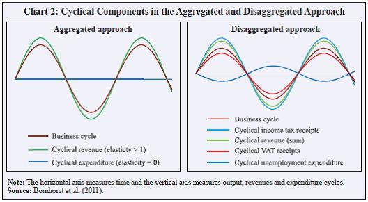

Accordingly, OECD has popularised computing CAB* by taking into account the component-wise break up of revenue and expenditure elasticities (Girouard and Andre 2005). Accordingly equations (3) and (5) get modified as:

R_i = ΣR_i* (Y/Y*) ^εi .......................................................................(7)

CAPB* = [ (ΣR_i (Y*/Y) ^εi ) – G (Y*/Y)ⁿ + X ] /Y * ......................(8)

where

Ri = actual tax revenues for the i-th category of tax

G = actual current primary government expenditures

ε_i = elasticity of revenue category i to output gap

n = elasticity of current primary government spending to output gap

X includes balances on account of all revenue and expenditure categories that do not require cyclical adjustment, for example, non-tax revenue, capital and net interest spending

OECD has also gone one step ahead and separated the revenue elasticity of output into two components -- an elasticity of tax revenue with respect to the relevant tax base, ε^{ri bi} and an elasticity of the tax base relative to a cyclical output indicator, ε ^{bi y} :

ε^{ri y} = ε^{ri bi} x ε ^{bi y} ...........................................................................(9)

Accordingly, revenue equation (7) gets modified into 10:

R_i = ΣR_i* [(Y/Y*) ^{εri bi} ] ^{εbi y}.....................................................................................................(10)

Substituting this into the CAPB equation, one can also get a revised equation (8). The IMF approach is simpler with minimum data requirements. OECD’s disaggregated approach, albeit more data intensive provides greater insights into the composition and extent of cyclicality of tax revenues and expenditures and hence enhances the stability and reliability of the results.

III.1.3 The ECB Methodology

The concept of a CAB has been at the centre stage in the revised EU framework for fiscal surveillance. With the 2005 reform on the Stability and Growth Pact (SGP), the budget balance adjusted for cyclical effects (along with other one-off and temporary measures, called structural balance) is the key indicator used for assessing country-specific medium-term fiscal objectives under the ‘preventive arm’ of SGP and of the fiscal adjustment imposed on member states in excessive deficit positions under SGP’s ‘corrective arm’. CAB allows for decomposing the fiscal position into the automatic reaction of the budget to changes in economic activity and the impact of a discretionary fiscal policy mostly in the hands of the government. The Fiscal Compact signed in March 2012 further reinforces the SGP framework by necessitating countries to adopt in their constitutions or other durable legislations a structural budget balance rule by 2014 (Mourre et al. 2013).

The ‘ECB approach’ is based on adjustments for output composition effects. While it is close to the OECD disaggregated cyclical adjustment, it differs from it in the sense that they separately estimate the cyclical components of individual tax and expenditure bases as well (Bouthevillain et al. 2001). The logic is as follows. When there are significant variations in the composition of output, using overall output gap as a measure of the cyclical state of an economy could have limitations. To understand its implications, we consider two scenarios of economic expansion, one consumption based and the other export driven economic, both implying the same output gap and hence the same level of cyclical adjustment. However, the actual fiscal impact of the same expansion may be more when the output gap is due to consumption driven expansion rather than being export driven assuming that the former is taxed more than the latter.

The difference arises because different components of GDP are bases to different types of taxes. For example, consumption and wage cycle may differ from overall business cycles and can also differ from each other, both in phases as well as amplitude (Chart 3). This might have different fiscal implications as wages are the base for income taxes while consumption is the base for indirect taxes. Hence, unlike equation (7), adjusted revenues can now be obtained as stated in equation (11):

R* = ΣR_i (B_i*/B_i) ^εi .....................................................................(11)

where B_i represents the relevant tax base for revenue category i. This kind of adjustment (that goes beyond business cycles) generates what we call structural revenues and the deficit so obtained after carrying out the necessary computations is called structural balances.

Studies for European economies have shown that controlling for changes in the composition of output changes the characterisation of fiscal policy in certain episodes (Bouthevillain et al. 2001). Applying the same methodology to South Africa (IMF 2006) shows that consumption and corporate profit growth rates beyond GDP expansion improve fiscal balances.

III.1.4 Adjustments beyond Business Cycles

While literature on this topic had initially started adjusting only for the business cycle impact on fiscal policy, over the years additional adjustments have also been made. Considering that our ultimate objective is to get an estimate of a true fiscal stance which is completely discretionary on the part of the government and is devoid of any macroeconomic fluctuations, there is a need to correct for any other shock or fluctuation that might influence fiscal balances on top of business cycles. Three additional kinds of adjustments have gained popularity: (i) the output composition effect, (ii) one-off effects that generate revenues/incurred expenditures on a temporary basis and (iii) changes in asset prices, commodity prices or terms of trade.

While the first one has already been discussed under the ECB approach, second one refers to cases such as large one-time revenues/expenditures due to spectrum sales, sales of concession rights, write-offs related to recapitalisation of banks and so on. This involves an easy adjustment as we need to take out this variable from the revenue and expenditure series and follow the usual step from (1) to (8) to arrive at CAB. However, in the absence of universally accepted standard criteria for identifying one-offs, it is advisable to use such adjustments carefully and sparingly.

The second kind of adjustment is based on the premise that commodity prices or real estate prices at times may rise temporarily due to surges in global demand or they may experience a price bubble or boom/bust cycle. The influence of that on fiscal revenues, if any, needs to be removed to determine the underlying fiscal position. This kind of adjustment is generally made for countries whose fiscal revenues are significantly dependent on commodities (terms-of-trade shocks). For example, in a copper-exporting country such as Chile, adjusting for this factor is important since otherwise a movement in copper prices might influence its fiscal policy in a wrong way. In the case of Spain, about 50-75 per cent of an increase in tax revenues between 1995 and 2006 was estimated to be transitory related to a continuing asset (housing) boom (Martinez-Mongay et al. 2007). Beginning 2008, the slump in Spain’s housing market exposed the vulnerabilities of Spanish fiscal accounts to movements in these asset prices. A study for the United Kingdom found that a permanent increase of 10 per cent in asset and house prices is estimated to increase the cyclically adjusted tax receipts directly by between 0.1 and 0.4 per cent of GDP annually (Farrington et al. 2008).

Taking into account asset price adjustments, revenue equation (3) stands modified as follows in equation (12):

R* = R (Y*/Y) ^εy (A*/A) ^εa ..........................................................(12)

where A*/A gives the asset price gap, deviation of asset prices from their benchmark level and ε_y is the elasticity of revenue to output gap and ε_a is the elasticity of revenue to asset price gap. If ε_a = 0, the equation reduces to the original one. It may be noted that while equation (10) is for aggregated revenues, it can also be suitably modified for disaggregated revenues as done before. The fiscal balance which is obtained by doing these additional adjustments for output composition, terms-of-trade shocks and one-off factors on CAB is called structural fiscal balance.

III.2 Country Experiences

Computing and analysing a cyclically adjusted/structural fiscal position is an integral part of fiscal/budget analysis units – the Ministry of Finance, Budget Office or Treasury in advanced countries like Canada, United Kingdom, United States and New Zealand. However, this is not a static process and they periodically undertake research to improve their cyclical adjustment methodology.

In the United Kingdom, the Office of Budget Responsibility (OBR) is responsible for assessing the effect of business cycles on public finances and it has been doing this based on a Treasury occasional paper (1995). The results of the analysis have, however, been periodically updated in 1999, 2003 and 2008. These were essentially based on the ‘one-step’ approach (akin to the IMF way) as they involved regressing public expenditure and receipts directly on the output gap. Since 2008, research has also focused on the two-step OECD approach, accounting for other adjustments like asset prices as well (Helgadottir 2012). The Government of Canada⁵ and the New Zealand Treasury have generally been computing CAB for their countries based on the OECD and IMF methodologies. Recent independent research has also tried to show that non-structural factors other than business cycles like asset prices could also be relevant for New Zealand (Parkyn 2010). To enhance transparency via computing structural balances while simultaneously managing uncertainty surrounding the computation of these balances, countries have attempted to give medium term forecasts using fan-charts for structural balances (through the use of sensitivity analyses and confidence intervals), for example, New Zealand and Canada (Parkyn 2010).

With an objective of strengthening fiscal frameworks towards achieving macroeconomic stability and given the close link between CAB and debt sustainability, countries have also adopted structural budget balance rules. Farrington et al. (2008) indicate that publishing cyclically-adjusted, or structural, forecasts of the budget balance and key fiscal aggregates help promote transparency in the operations of fiscal policy and enhance the credibility of fiscal consolidation. Hence, there is an argument in favour of setting up fiscal rules in terms of CAB and not general balances as in the case of EU, Australia and UK as targeting CAB tends to improve the stabilizing properties of the rule, that is, making it more counter-cyclical (Bova et al. 2013).⁶ Bova et al. (2013) show that for advanced economies the introduction of a cyclically-adjusted balance as the target for the rule has been associated with less procyclical public spending.

Amongst emerging economies there is extensive research for Latin American economies. Studies both within and outside governments have estimated the cyclically adjusted budget balances of governments as an alternative fiscal indicator that can contribute to a more effective fiscal policy and fiscal analysis. Studies have tried to compare the extent of discretionary fiscal stance and impulse across different Latin American countries during different crisis episodes and across different initial debt levels (Daude et al. 2010). Some of them like Chile, Columbia and Panama have adopted structural balance based fiscal rules as well after extensive research in the field.⁷ For Chile, procyclicality is found to be lower following the adoption of the structural balance rule only after excluding the years of the financial crisis (Bova et al. 2013). Brazil, (one of the BRICS nations to which India is frequently compared) has been computing and constantly updating its CAB estimates using both the OECD and the IMF methodologies during 2000s whereby budget balances are adjusted for cyclicality of GDP and oil revenues (Gobetti et al. 2010; Oreng 2012). CABs have also been computed for South Africa using the OECD disaggregated approach and HP filter based potential output (South Africa see, IMF, 2006).

III.3 Indian Literature

Fiscal stance in India is analysed by policymakers and academicians using the headline fiscal balance. Although vast at the global level, comprehensive research on adjustment of fiscal balances for business cycles and other non-structural parameters is rather limited in India. In India literature on assessing fiscal policy has focused on slightly different angles. While many studies are devoted to assessing the procyclical nature of the Indian fiscal policy, assessing the sustainability of India’s debt levels has also been popular among researchers (Kaur et al. 2014; RBI 2013). Research has also focused on broader macro-stabilisation issues like the impact of fiscal deficit on growth and inflation. While empirical evidence does point towards some crowding-in impact of public investments, particularly capital expenditure mostly in the infrastructure sector (Kumar and Soumya 2010; Mundle et al. 2011; RBI 2001), empirical evidence with regard to the impact of fiscal deficit on inflation is rather inconclusive. With regard to computing CAB for India, some preliminary analysis was done for the 1980s and 1990s, simply by applying the HP filter on the revenue and expenditure series to get the cyclically adjusted fiscal variables or with a different objective to show the small size of the cyclical deficit (Rangarajan and Srivastava 2005; RBI 2001). Another attempt to compute CAB for India was done in the mid-2000s with the prime objective of analysing the impact of macroeconomic performance on structural revenues for India (Pattnaik et al. 2006).⁸ Even when India adopted a fiscal rule, it was preferred to be an overall rule, rather than in cyclically adjusted terms.

Some domestic evidence/anecdotes in the Indian context, particularly post the global financial crisis enunciate the need to focus on fiscal balances adjusted for cycles. While in general there is evidence favouring procyclicality of India’s fiscal policy over a long term, there seems to be a reduction in the extent of procyclicality of India’s fiscal policy in recent time periods as the central government undertook significant counter-cyclical measures during the 2008 downturn accompanying the global financial crisis (RBI 2013). The extent of automatic stabilisers was estimated to be about 0.5 per cent of GDP for India in 2008-09 (RBI 2009). While this was on the lower side when compared to advanced economies, it was comparable with other EMEs. The only standard attempt to quantify CAB for India used the IMF aggregate methodology and estimated the desired elasticity parameter (albeit at an aggregate level) for India at 1.5. It showed that after initial success in containing CAB around 2006-07, it increased considerably during the crisis period. Notwithstanding an increase in (positive) output gap in the post-crisis period (2009-11) and subsequent increase in inflation, CAB continued to be expansionary with limited withdrawal of the expansionary stance, albeit a reduction in fiscal impulse (Misra and Ghosh 2014). However, analysing the structural component of fiscal balance for India using the standard OECD/ECB approach has not been attempted.

More importantly, in recent times, the Government of India has also shown some inclination towards analysing fiscal policy independent of cycles. The Economic Survey (2013-14) (Government of India 2014) observed ‘…fresh thinking on a responsible fiscal policy framework is required. This should feed into a new FRBM Act. The modified Act needs to take into account business cycles and have penalties that are strong enough so that it cannot be ignored.’ Economic Survey (2014-15) (Government of India 2015) went a step ahead and categorically included cyclical considerations and one-off factors as short term issues in the fiscal framework. It says that with growth reviving and macroeconomic pressures abating for India, there is a need for using fiscal policy as a cushion.

Section IV
Estimation of CAB for India

For any calculation of structural balance, two parameters need to be estimated. The first is the trend and cyclical components of GDP and of the proxy tax bases and asset prices if the disaggregated approach is used. The second is determining tax elasticities of different revenue and expenditure items with respect to output gap.

IV.1 Computing Potential Output

Three different potential output estimates have been computed so as to ensure the robustness of the results – the Hodrik Prescott (HP) filter, the Band Pass (BP) filter of Christiano-Fitzgerald (CF) and the production function approach. While the first two are univariate filters and hence used extensively, (Bornhost et al, 2012; Misra and Ghosh 2014), the production function approach (used by OECD) is based on a theoretical foundation although it suffers from large scale data issues.

IV.1.1 The HP Filter

The filter balances between its proximity to original series and the smoothness of the filtered series.⁹ The HP filter is the simplest of all filters and does not require any economic judgment. Implementing the HP filter, however, requires an appropriate choice of the smoothening parameter, λ.¹⁰ Another important practical issue in implementing the HP filter is the end-point bias. HP filtering amounts to deriving the trend series {x_t^*} as a moving weighted average of actual observations with symmetrically distributed and decreasing weights. In finite samples, the distribution of weights becomes highly asymmetric at the end points; excessively large weights are attributed to extreme observations. The calculated trend values at the extremes of the sample are therefore artificially close to actual observations, and the cyclical component of the series is correspondingly underestimated. To alleviate end-point bias, it is common to complement the sample with forecasts, even though a substantial bias seems to remain.

An alternative to the HP filter is also obtained by setting the smoothening parameter value using the frequency power rule of Ravn and Uhlig (RU) (2002). While Hodrick and Prescott recommend the value 2, Ravn and Uhlig recommend the value 4.

IV.1.2 The BP Filter

Band Pass filters are considered more ideal as they isolate the cyclical component of a time series by specifying a range for its duration (Baxter and King 1999). A BP filter is a linear filter that takes a two-sided weighted moving average of the data where cycles in a ‘band’, given by a specified lower and upper bound, are ‘passed’ through, or extracted, and the remaining cycles are ‘filtered’ out. To employ a band pass filter, the user must first choose the range of durations (periodicities) to pass through. The range is generally described by a pair of numbers, specified in units of the workfile frequency.¹¹ There are different variants of band pass filters available in most software packages. While the fixed length filters use the same number of lead and lag terms for every weighted moving average, it loses observations from both the beginning and the end of the original sample equal to the number of lags. The asymmetric filter is more general with time-varying weights, both depending on the data and changing for each observation; the asymmetric filtered series do not have this requirement and can be computed to the ends of the original sample. EViews computes the Christiano-Fitzgerald (CF) form of this filter (Christiano-Fitzgerald 2003).

IV.1.3 Production Function Method

While IMF uses the HP filter based output gap measures, OECD uses the production function framework. The main advantage of the production function framework is a clear link to economic theory, which allows an understanding of the driving forces behind the path of potential output. Generally a two factor Cobb-Douglas production function of the form given in equation (14) is used owing to its reasonable simplicity and transparency.

Y = TFP . L^α . K^(1-α)....................................................................(14)

where Y = real GDP; L = actual labour input; K = actual capital stock; TPF = total factor productivity; α = average labour share.

Or in natural logarithms:

lnY = ln TFP + α lnL + (1 – α) lnK..........................................(15)

Equation (15) is used to derive total factor productivity in the whole economy by substituting observable variables in the equation and calculating TFP as a residual.

Potential output is calculated by combining smoothened (HP filtered) series of total factor productivity, capital stock and employment, using the same production function (Mishra 2013) as shown in equation (16).

lnY*= lnTFP* + α lnL* + (1 – α) lnK*....................................(16)

where * indicates that the series is at its trend or potential level.

IV.1.4 Estimation of Potential Output for India

This paper uses the first two approaches to obtain the potential output for GDP. It uses annual GDP data at factor cost at current and constant prices as given by CSO for the period 1970-71 till 2014-15. Since February 2015, a new GDP series (base 2011-12) has been released by CSO. Given that the back series to this are not available at this stage, a suitable back series has been created by using the average for 2011-12 and 2012-13 as the linking factor. Along with the new series, potential output was also computed using the old series (2004-05 = 100). Considering that the old series stops at 2013-14, again the average for 2011-12 and 2012-13 was used to obtain the GDP number for 2014-15 so that the old series is complete.¹²

In order to avoid end-point bias in most statistical filters, data are projected forward for two years using RBI forecasts of 7.5 per cent for 2015-16 and 2016-17 (about 13 per cent in nominal terms, assuming 5.5 per cent inflation). For the HP filter, standard smoothening parameter for annual data of 100 is used. The potential output growth rates as well as the output gap (actual minus the potential divided by potential GDP growth rates) given by all the three measures (HP, RU and BP) are reported in Annexure I. This has been done for both the old and new series.

IV.2 Estimation of Elasticities for India

As stated earlier, elasticities can be analysed either at the aggregate level (as used by IMF) or in a more disaggregated manner (the OECD way). Generally a unit elasticity for revenue receipts to output has been assumed for India for convenience (IMF Fiscal Monitor, various issues; Pattnaik et al. 2004). Few attempts have been made to compute empirically the revenue elasticity at the aggregate level. These attempts have generally arrived at an elasticity greater than one (Misra and Ghosh 2014; Mundle et al. 2011). While it is considered appropriate to use a regression based approach for computing elasticity and it is extensively used for advanced economies it is avoided in view of frequent changes in tax laws in emerging economies (Bezdek et al. 2003). Another hindrance is lack of data on tax bases for emerging markets.

Certain Latin American and some oil exporting emerging economies have started estimating these elasticities. Among BRICS nations there is empirical evidence only for Brazil and South Africa. Recognizing that elasticities of revenues to output gap may differ across different types of taxes and true cyclical adjustment should try and capture the cyclicality amongst various taxes the OECD disaggregated methodology has been adopted in this paper to compute elasticities. The two-step approach also avoids the need to create a policy-adjusted tax revenue series, which is difficult to construct and prone to measurement errors, making the econometric results more robust. Moreover, this OECD approach while used adequately in case of other countries has never been tested on Indian data. Notwithstanding the advantages of using the disaggregated approach, it can also have limitations. This approach can only be used where we can clearly identify the tax base for which data are available for a reasonable period to estimate and check the sensitivity of the particular tax category. Also, the various taxes should be exhaustive enough to cover a large part of the overall tax receipts. Otherwise this method could underestimate cyclicality if various components are left out for lack of tax base information.

IV.2.1 Ascertaining the Tax Base

The starting point for this approach is identifying which taxes can have a cyclical element and whether data on tax bases are available. Looking at the Indian fiscal data, the overall revenues can be broken into tax and non-tax revenues, with the former being more dominant and elastic with respect to output gap. Tax revenue can be further disaggregated into direct taxes comprising largely of personal income tax and corporate tax and indirect taxes comprising of excise and customs duties. With regard to the base for each of these taxes, wages and salaries and compensation to employees are generally used as the base for income tax and corporate earnings/profits and gross operating surplus are used as the base for corporate taxes (Bouthevian et al. 2001; Parkyn 2010). Getting information on suitable tax bases has been a constraint for EMEs. While Brazil uses wages as the base for income tax, it retains GDP as the base for corporate tax in the absence of a suitable base for the latter (Oreng 2012). In the search for a suitable proxy for wages and salaries in India, this study arrived at data on ‘compensation to employees’ as provided by National Accounts Statistics (NAS). The only problem is that this information is available with about a 2-year lag. Information on corporate earnings/profits for India was available from CMIE/Prowess only since the late 1990s and that rules out any meaningful regression because of inadequate data points. Hence, as a proxy, ‘private income’ as given by National Account Statistics was used.¹³

For indirect taxes, the most common base used is private consumption (ECB, OECD, New Zealand) although countries have also used variants like retail sales (Brazil). In this study we have broken down indirect taxes into its two major components – excise and customs duties - recognizing that the base is different for the two. For excise duties, two tax bases were considered: First, private consumption as per international practice and second, manufacturing GDP, as used in India to compute buoyancy estimates (Mid-Year Review of the Government of India, October 2014). For customs duties, ‘trade’ (sum of exports and imports) was considered a suitable base. The choice of tax base was influenced by international literature, domestic practices and availability of data.

For some components no cyclical adjustment was done and they were taken as is. These include non-tax revenues—in India mainly interest receipts and dividends (potentially cyclical but quite volatile). In the entire literature on cyclical adjustments, the only expenditure component for which cyclical adjustments are done is social security contributions like unemployment insurance. Since this component for all practical purposes does not exist in the Indian case, no cyclical adjustment of expenditure was done.¹⁴ Data on actual fiscal revenues and expenditures and GDP and its components from 1970-71 to 2013-14 as given in the Handbook of Statistics of the Reserve Bank of India and the CSO website respectively were used. The data for 2014-15 are revised estimates based on Union Budget 2015-16. All the variables are in real terms. While data on most tax bases are available in real terms, fiscal variables were converted into real terms mostly by deflating the revenue and expenditure items using a deflator based on the tax base.¹⁵

IV.2.2 Estimation of Elasticities for India using the Two-step Method

As given in equation (5), two elasticities need to be computed: (i) elasticity of tax revenues with respect to the relevant tax base, and (ii) the elasticity of tax base relative to output gap. The elasticities essentially relate to the percentage change in one variable, X, to a one-percentage-point change in another variable Y. It can be computed using the standard log-log regressions. In this case, the best way is to regress the particular revenue on its base and then the base on the output gap variable. However, most revenue series and their bases are observed to be I(1) series and the output gap series are generally I(0) as given in Table 1.

To address econometric limitations, emerging markets, particularly BRICS have generally relied on elasticities based on regressions of different variants.¹⁶ With regard to the first elasticity, that is, tax revenue on tax base, the standard log-log regression was used regressing tax revenues on proxy tax bases in a co-integrated framework recognizing both series are I(1) (for Brazil see Oreng 2012), or using a log-difference specification (South Africa, 2006). In a generic notation form, this can be written as:

log R_i = c + ε_RiBi · log B_i + u .....................................................(17)

d(log R_i) = c + ε_RiBi · d (log B_i) + u...........................................(18)

Results of equation (17) for India are reported in Table 2 and in Annexure II. The elasticities are all significant at the 1 per cent level of significance.

With regard to the second elasticity, tax base on output cycle, different approaches have been used to tackle the stationarity problem. First, assuming that cyclical elasticities are unchanged in equilibrium, use of both levels or cycles as regressands are considered to be consistent with the structural balance assumption (for Brazil see Oreng 2012). Hence, the standard log-log regressions in levels are performed to obtain the long term elasticities after certifying for the presence of unit root and in a co-integrating framework by ensuring that the residuals are stationary (as given by equation 19). The second approach involves the use of cycles (as shown by equation 20). The base cycles are regressed on output cycle in log terms (at times in first difference as well) to get the elasticities (South Africa see IMF 2006).

log B_i = c + ε_BiY · log Y + u ……………………….. (19)

log (B_i/B_i*) = c + ε_BiY · log (Y/Y*) + u ……………. (20)

In computing the elasticities care was taken to ensure that both methods made sense econometrically. While the first method scores over the latter in simplicity, the second method captures the revenue sensitivity to output gap exactly albeit involving large scale use of trend filtering techniques, which has its limitations. Results of the elasticity estimates for India based on this regression are reported in Table 3.

The problem of endogeneity generally figures in any discussion on elasticity. It may be noted here that use of the OECD two-step approach tackles this issue to some extent as we regress particular revenues on their bases rather than on output. However, some amount of endogeneity still prevails because of the second step of the regression (tax base on output gap). One possible method for addressing this issue is to estimate the equation using instrumental variables. But in practice it can often be difficult to identify strong instruments for domestic GDP. This was the approach used in the UK Treasury’s 2008 working paper, using the world output gap and world interest rates as instruments. This detected no significant evidence of bias which is in line with Darby and Melitz’s (2008) conclusions. Just to check the robustness of the results, one period lagged GDP was used as an instrument. It was observed that there was not much difference in the coefficients so obtained. In fact for the regression of compensation to employees’ gap on lagged output gap, the elasticity was a tad higher than what is reported.

An alternative being used in literature is an elaborate structural vector autoregressive model (SVAR) to empirically analyse the relationship between fiscal and economic shocks (Blanchard and Perotti 2002). While this approach has the advantage of being grounded within an economic model with behavioural foundations which allows for bi-directional feedback between fiscal policy and economic activity, it does not lend itself to producing direct estimates of the structural budget balance (Parkyn 2010). It can at best be complementary to the analytical approach mentioned earlier and followed in this paper.¹⁷ However, considering that this is the first ever attempt in the Indian case to do disaggregated adjustments, simplicity has been preferred.

The product of the two elasticities (revenue with respect to base and base with respect to output) will give us the final value of the sensitivity of the particular category of revenue items to GDP. These are reported in Column (4) of Table 4. As can be seen from the table, there are significant differences in elasticity estimates across tax categories thus justifying the use of a disaggregated analysis in the Indian context. This also shows that while zero expenditure elasticity may be a reasonable approximation in the Indian case given the lack of social security contributions and unemployment benefits, using the rule of thumb of revenue elasticity of one might be too simplistic in any analysis of this kind and may understate the contribution of the automatic component.¹⁸ As expected, the elasticities are higher for personal income and corporate taxes as they are progressive.

While elasticity estimates are given over a range in Column (4) (Table 4), for further analysis we used the upper limit of the range. It may be noted here that a higher estimate for elasticity implies attributing too much variation in the business cycle and thus underestimating structural change. Though not strictly desirable technically, this deserves some policy merit. In attempting to bring a medium-term perspective to fiscal policy, it may be better to use a higher estimate to assess the sustainability of fiscal settings. Compared to monetary policy, fiscal policy tends to change at less frequent intervals, it has longer lags in implementation and is harder to unwind policy loosening (that is, there is a deficit bias induced by the political economy). This may mean that at least in boom times it may be prudent to use higher elasticity estimates so as to avoid the likelihood that discretionary fiscal deficit is understated requiring difficult policy reversal later (Parkyn 2010).

Given the lack of previous work applying this disaggregated approach to Indian data, the results were compared to OECD estimates and to other EMEs which have such information (Table 5).¹⁹ Estimates from disaggregated models clearly bring useful insights. They point out the elastic nature of India’s income and corporate taxes. While India’s elasticity estimates for indirect taxes are below international levels, direct tax elasticities are much higher than that of advanced countries and are closer to BRICS countries. India’s indirect tax elasticities are slightly lower than even other BRICS nations for which estimates are available. This hints at a policy priority to enhance elasticity of indirect taxes in India.

Section V
Estimation of Structural Balance: Empirical Results

V.1 Adjustment for Business Cycles Impact (the OECD Methodology)

Using the potential output and elasticity estimates computed in the previous section, the cyclically adjusted primary balances for India based on the OECD disaggregated approach are then computed using equation (8). The cyclically adjusted fiscal deficit so obtained is shown in Chart 5 for the post-1990s period²⁰.

V.2 Output Composition Effect (ECB Methodology)

In line with Bouthevillain et al. (2001), the HP (smoothening parameter of 100) and BP filters (Christiano-Fitzgerald type) were used to estimate the gap measures of each of the following tax bases: Compensation to employees, private income, manufacturing GDP, private consumption and trade. The gap estimates for HP filter are shown in Chart 4.²¹ The corresponding correlations with overall GDP are given in Table 6. Clearly, if the gap measure of the base differs significantly from the overall GDP output gap (reflected in lower correlations), it indicates the presence of the output composition effect. Chart 4 and the correlations in Table 6 indicate the presence of the composition effect. While the direction of output cycle and tax base cycle remain the same (reflecting positive correlations), it is less than perfect (less than one). A lower correlation of output gap with compensation to employees’ gap is in line with the results of other countries as well reflecting sluggish labour market adjustments (Helgadottir et al. 2012; IMF 2006). While manufacturing GDP and private income seem to have a cycle with a higher amplitude than the output cycle, the private consumption cycle approximates the output cycle the closest.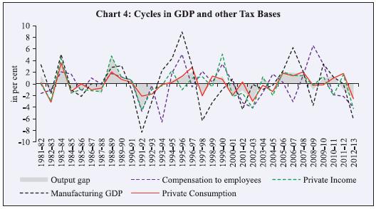

V.3 One-off Factors

As indicated in Section III.1, computing one-offs can be very subjective. To bring in some objectivity into computing one-offs across nations, the European Commission has spelled out some principles to identify one-off measures (Borhost et al. 2011; Larch and Turrini 2009):

1. Size (only measures having a significant impact, assumed to be above 0.1 per cent of GDP on the general government balance should be considered;

2. Duration (the impact of one-offs should be concentrated in one single year or a very limited number of years); and

3. Nature (one-offs are typically, but not exclusively, included as capital transfers).

Looking at the Indian case, we include all the non-debt capital receipts such as disinvestment proceeds, small savings/provident fund and recovery of loans as part of revenue to compute the primary balance. However, international institutions like the IMF keep some of these non-debt capital transfers out of the structural balance computation.²² Logically also one needs to exclude disinvestment proceeds from capital receipts since these are one-off receipts which result in forgoing future revenue from disinvested shares, just as borrowings imply interest payments. However, any comparison of structural balance with official estimates is impossible without inclusion of these capital transfers which is a practice followed in our budget. Notwithstanding these limitations in the Indian context, some obvious adjustments were made to the Indian revenue data to decide on the one-offs. Arbitrariness was avoided by basing it on the criteria mentioned by Larch and Turrini (2009) of size, duration and nature. Items were recognised as one-off factors in the Indian context post-1990s and accordingly adjustments were made to exclude: First, recovery of loans for 2002-03, 2003-04 and 2004-05 which includes receipts from states under the Debt Swap Scheme amounting to ₹137.66 billion, ₹462.11 billion and ₹436.75 billion respectively satisfying all the three criteria. Second, disinvestment receipts and total capital receipts of 2007-08 which includes ₹343.09 billion under miscellaneous capital receipts which represents the Reserve Bank’s surplus transferred to the central government on account of transfer of its stake in SBI to the central government. This satisfies the criteria of duration and nature. Third, sale of spectrum, which is also a one-off receipt (included as part of non-tax revenue) which is also excluded based on size and duration criteria.

V.4 Official and Structural Balances for India: Analysis of Results

The final structural balance series for India, obtained by accounting for business cycles, output composition effect as well as one-off factors using equations (8) and (9) is given in Chart 5. For better comparability with official estimates and better clarity, the average structural balance as obtained using different potential output estimates is used in this chart.²³ As can be seen from Chart 5, the presence of cyclical and output composition effects are the most prominent post-2000s. Table 7 shows the effect of business cycles, output composition and one-off effects on official primary deficit for 2006-14.²⁴

Chart 5 shows that while during the early 2000s cyclical factors worsened the primary fiscal balances during the high growth phases of 2006-07 and 2007-08, cyclical factors contributed positively to the overall primary balance with both official as well as structural balances recording surpluses (hence, the negative sign for the fiscal deficit in the Chart). Post 2008-09, however, the fiscal stimulus withdrawal was less than that shown by official figures (Table 7). Since 2008-09, the fiscal position has remained under deficit mode. Adjusting for the growth slowdown and consequent below potential growth during 2008-09, deterioration in primary surplus was lower than what was given in official figures by about 0.4-0.5 per cent. Since 2009-10 when growth revived, the cyclical component worked in the opposite direction with structural deficit being higher than the official one by more than 0.8 per cent on an average based on range of potential output estimates. This implies that withdrawal of fiscal stimulus was actually lower than what was shown in official figures during this period.²⁵ Since then, however, fiscal consolidation seems more credible, even though there are issues about the quality of expenditure which are beyond the scope of this paper.

Based on this analysis the average automatic stabiliser component turns out to be about 0.6-0.7 per cent during the last decade. Moreover, the output composition effect could be another 0.2-0.4 per cent of potential GDP. Although lower than the figures for advanced countries, these are comparable to other emerging market counterparts and are high enough not to be ignored.

With regard to disinvestment proceeds, recognizing that they are truly revenue generating, in 2005-06 to 2008-09 the disinvestment proceeds were not used for financing budgetary expenditure but were credited to the National Investment Fund (NIF) constituted in 2005. The returns on investments from NIF were treated as non-tax revenues to be used for financing expenditure on social infrastructure and providing capital to viable PSUs. Since 2009-10, however, the government has been using the divestment proceeds to finance programme expenditure. Taking disinvestment proceeds out of the non-debt capital receipts since 2009-10 is estimated to increase the structural deficit by another 0.2 to 0.3 per cent of potential GDP.

V.5 Adjustment for Asset Prices

While this paper tried to capture the impact of output cycles, tax base cycles and one-off factors, no correction for the asset price cycle has been undertaken. This was considered reasonable in view of two factors: First, asset price cycle adjustment is based on the premise that boom/bust cycles in commodity prices or real estate prices may influence fiscal revenues, and that needs to be removed to determine the underlying fiscal position. In literature on emerging markets, this kind of adjustment is generally made for countries whose fiscal revenues are significantly dependent on commodities such as copper-exporting country like Chile and oil revenues in the case of Brazil (Oreng 2012) and other Gulf countries. Countries have also avoided such adjustments in view of the modest contributions of asset prices to the fiscal sector (South Africa, 2006) or have observed that asset and commodity prices are not significant in explaining the deviation of revenue from its cycle for South Africa (Aydin 2010). The Indian case is similar. Second, if at all any asset prices are considered suitable for cyclical adjustments it will be housing prices on which time-series data are not available for a reasonably long period to conduct any analysis.²⁷

Section VI
Conclusions and Future Scope of Work

Although empirical work in the area of structural fiscal balance on the lines conducted for other countries is rather scarce for India, the concept as such has been gaining importance. The last few Economic Surveys and Mid-Year Reviews released by the government and the recent Union Budget have hinted at the need for analysing fiscal policy by taking into consideration business cycles and credit cycles etc so as to get a picture of the durable nature of fiscal correction. This paper makes an humble attempt to empirically compute the automatic impact of cycles on fiscal policy. Considering that India also has different cycles for different components of revenues, it tried to estimate the structural balances as well. This will enable us to examine whether change in output composition influences the fiscal balance or not and accordingly whether one should be bothered about it while formulating policies. The robustness of results was ensured by using a range of potential output estimates and checking elasticities for sub-sample periods.

The main findings of this study are: (i) there are significant differences in the elasticities of various tax revenues with respect to output gap as estimated using the OECD disaggregated approach. These are estimated to be in the range of 0.5-2.4 using a range of potential output estimates, (ii) the automatic component of fiscal balances could be in the range of 0.6-0.7 per cent, adjusting for one-off factors, and (iii) the impact of changes in composition of demand using the ECB approach on fiscal balances was found to be another 0.2-0.4 per cent of GDP.

As the literature indicates, computing structural balances and its use for policy purposes has been an area of on-going research both for countries that have adopted it in their fiscal rules and even for other countries which use this concept to get a better assessment of their fiscal policies. Further research in this area can explore: (i) improvising the computation of potential output estimates using the production function approach, (ii) getting the maximum disaggregated and most precise elasticity parameters via dissociating service tax elasticity, elasticity of some non-tax revenues (if possible like dividends and profits), using the SVAR method to compute elasticities that can complement the OECD approach (if not as a substitute), and (iii) explore the role of asset prices in fiscal revenues that has off late gained increasing attention from institutions which conduct fiscal surveillance (such as IMF, OECD and European Commission). The two channels through which asset price movements can get transmitted to fiscal revenues are through changing the tax base either directly via capital gains or transaction taxes and indirectly through wealth effects. While the share of the former is less in India and the latter is not so important at this stage, these effects are on a rise with housing assets increasingly acquiring a larger share of household wealth in India.

References

Aydın, Burcu (2010), ‘Cyclicality of Revenue and Structural Balances in South Africa’, IMF Working Paper, WP/10/216, September.

Baxter and King (1999), Measuring Business Cycles, approximate band pass filter for economic time series. University of Virginia

Bezdek, V., K. Dybczak, & A. K. Krejdl (2003), “Czech Fiscal Policy: Introductory Analysis” Working Papers 2003/07, Czech National Bank, Research Department.

Blanchard, Olivier and Roberto Perotti (2002): “An Empirical Characterization of the Dynamic Effects of Changes in Government Spending and Taxes on Output”, Quarterly Journal of Economics

Bornhorst, Fabian, D. Gabriela A. Fedelino, J. Gottschalk and T. Nakata (2011), ‘When and How to Adjust Beyond the Business Cycle? A Guide to Structural Fiscal Balances’, Technical Notes and Manuals 11/02, Washington DC: International Monetary Fund.

Bouthevillain, Carine, C.T. Philippine, V.D. Gerrit, Pablo Hernandez de Cos, G. Langenus, Matthias Mohr, Sandro Momigliano and Mika Tujula (2001), ‘Cyclically adjusted Budget Balances: An Alternative Approach’, ECB Working Paper No. 77.

Bova, Elva, Nathalie Carcenac and Martine Guerguil (2013), ‘Fiscal Rules and the Procyclicality of fiscal policy in the developing world’, IMF-World Bank Conference on Fiscal Policy, Equity and Long-Term Growth in Developing Countries, Washington DC, April 21-22.

Brown, Car E. (1956), ‘Fiscal Policy in Thirties: A Reappraisal’, American Economic Review, 46 (5): 857-879.

Budina, Nina, Tidiane Kinda, Andrea Schaechter and Anke Weber (2012), ‘Fiscal Rules at a Glance: Country Details from a New Dataset’, IMF Working Paper, November.

Christiano Lawrence J. and Terry J. Fitzgerald (2003), “The Band Pass Filter”, International Economic Review, Volume 44, Issue 2, pages 435–465, May.

Darby, J. and Melitz, J. (2008), “Automatic stabilisers”, Economic Policy, October 2008

Daude, Christian, Angel Melguizo and Alejandro Neut (2012), ‘Fiscal Policy in Latin America: Counter cyclical and sustainable at last?’ OECD Development Centre, Working Paper No. 291.

Debrun, Xavier and Radhicka Kapoor (2012), ‘Fiscal Policy and Macroeconomic Stability: New Evidence and Policy Implication’, Revista deEconomía yEstadística,CuartaÉpoca, 48 (2) (2010): 69-101.

Farrington, Stephen, John Mc Donagh, Catherine Colebrook, and Andrew Gurney, 2008, “Public Finances and the Cycle,” Treasury Economic Working Paper No. 5 (Washington: International Monetary Fund).

Fedelino, Annalisa, and others (2009), ‘Computing Cyclically Adjusted Balances and Automatic Stabilizers,’ Technical Notes and Manuals. Washington DC: IMF.

Girouard, Nathalie and Christophe Andre (2005), ‘Measuring Cyclically Adjusted Budget Balances for OECD Countries’, OECD Economics Department Working Paper No. 434. Paris: OECD.

Gobetti, Sergio Wulff, Raphael Rocha Gouvêa and Schettini, Bernardo Patta (2010), ‘Structural Fiscal Balance: A Step Towards The Institutionalization of Anti-cyclical Policies in Brazil’, Discussion Paper No. 1515, IPEA Instituto de Pesquisa Econômica Aplicada. Available at: http://www.ipea.gov.br

Government of India (2014), Economic Survey 2013-14. New Delhi: Ministry of Finance, pp. 39.

--------------------- (2015) Economic Survey 2014-15. New Delhi: Ministry of Finance, Vol I pp. 49.

Helgadottir, Thora, Graeme Chamberlin, Pavandeep Dhami, Stephen Farrington and Joe Robins (2012), ‘Cyclically adjusting the public finances’, Office of Budget Responsibility, Working Paper No.3, June.

Heller, Peter S., Richard D. Haas and Ahsan S. Mansur (1986), ‘A Review of the Fiscal Impulse Measure’, IMF Occasional Paper No. 44.

Hodrik, R. J. and E. C. Prescott (1997), ‘Postwar U.S. Business Cycles: An Empirical Investigation’, Journal of Money, Credit, and Banking, 29: 1–16.

Horton, Mark and Asmaa El-Ganainy (2012), ‘Fiscal Policy: Taking and Giving Away’, IMF, Finance & Development, March.

International Monetary Fund (2006), ‘Cyclically Adjusted Budget Balances: An Application to South Africa’, in “South Africa: Selected Issues,” IMF Staff Country Report 06/328, Chapter IV.

Kumar, Rajiv and Alamuru Soumya (2010), ‘Fiscal Policy Issues for India after the Global Financial Crisis (2008-2010)’, ADBI Working Paper Series, September.

Larch, Martin, and Alessandro Turrini (2009), “The Cyclically adjusted Budget Balance in EU Fiscal Policy Making: A Love at First Sight Turned into a Mature Relationship,” European Commission Policy Paper 374 (Brussels: European Commission).

Martinez-Mongay, Carlos, Luis-Angel Maza Lasierra and Javier Yaniz Igal (2007), ‘Asset Booms and Tax Receipts: The Case of Spain, 1995–2006’, Directorate-General for Economic and Financial Affairs, European Economy: Economic Papers No. 293.

Matier, Chris (2011), ‘A comparison of Finance Canada and PBO Estimates of the Government of Canada’s Structural Budget Balance’,, Ottawa, Canada, December. Available at: www.parl.gc.ca/pbo-dpb

Mishra, P. (2013), ‘Has India’s Growth Story Withered?’, Economic and Political Weekly, February.

Misra, S. and Ghosh (2014), ‘Quantifying the Cyclically adjusted Fiscal Stance for India’, RBI Working Paper, February.

Mourre, Gilles, George-Marian Isbasoiu, Dario Paternoster and Matteo Salto (2013), ‘The cyclically-adjusted budget balance used in the EU fiscal framework: an update’, European Commission, Economic Papers 478, March.

Mundle, Sudipto, N.R. Bhanumurthy and Surajit Das (2011), ‘Fiscal consolidation with high growth: A policy simulation model for India’, Economic Modelling, 28: 2657–668.

OECD (2016),”Economic Policy for Reforms: Going for growth”, Interim Report, April.

Oreng, Mauricio (2012), ‘Brazil’s structural fiscal balance’, Working Paper No.6, ITAU, April.

Parkyn, Oscar (2010), ‘Estimating New Zealand’s Structural Budget Balance’, New Zealand Treasury Working Paper 10/08, November.

Pattnaik, R. K., Deepa S. Raj and Jai Chander (2006), ‘Fiscal Policy Indicators in a Rule Based Framework: An Indian Experience’, Paper presented at Bank Italia Conference, April.

Quinet, A. and K. Bouthevillain (1999), ‘The Relevance of Cyclically-Adjusted Public Balance Indicators — the French Case’, in Indicators of the Structural Budget Balances. Banca d’Italia, pp. 325-352.

Rangarajan, C. and D.K. Srivastava (2005), ‘Fiscal Deficits and Government Debt in India’, NIPFP Working Paper No. 35, July.

Ravn Morten and Harald Uhlig (2002), “On adjusting the Hodrick-Prescott filter for the frequency of observations”, The Review of Economics and Statistics, 2002, vol. 84, issue 2.

Reserve Bank of India (2013a), Report on Currency and Finance, 2009-12.

---------------------------(2013b), Annual Report, 2012-13

-----------------------------, Report on Currency and Finance, 2000-01.

Roger, W. and H. Ongena (1999), ‘The Commission Services’ Cyclical Adjustment Method’, in Indicators of the Structural Budget Balance. Banca d’Italia, pp. 71-96.

Sancak, Cemile, Ricardo Velloso and Jing Xing (2010), ‘Tax Revenue Response to the Business Cycle’, IMF Working Paper WP/10/71, March.

* Smt Sangita Misra is Assistant Adviser in RBI’s International Department and Dr Pushpa Trivedi is Professor & Institute Chair Professor, Humanities and Social Sciences Department, Indian Institute of Technology, Bombay. The authors are thankful to Prof. Tara Shaw, IIT, Mumbai and to an anonymous referee for valuable observations on the paper. The views expressed by the authors are personal and not of the institutions they belong to. Usual disclaimers apply.

¹ The difficulty surrounding the estimation of the unobserved potential-output to assess the impact of business cycles and the conventional belief of negligible automatic stabilisers in developing economies have somewhat prevented the exploration of this area.

² Of course, it does not exactly work in that way in countries like India.

³ It may be noted that R = R* if Y=Y*.If, however, the economy is booming, that is, Y ≥ Y* implies R ≥ R* leading to more revenue generation and vice versa.

⁴ It may be noted that since IMF’s definition is expressed in terms of balances, excluding interest payments this is essentially tantamount to adding interest payments to overall balances to get primary balances: PB=OB+INT.

The same definition when expressed in terms of deficit, as usually used in India, primary deficit will equal overall deficit less interest payments. Both the definitions are consistent.

⁵ Canada provides two estimates of CAB – one from Finance Canada and another from the Parliamentary Budget Office that generally provides independent analyses to Parliament on the state of the nation’s finances (Matier 2011).

⁶ Italy, for example, did extensive research in the field of structural balances before adopting a structural balance based fiscal rule. Though the European Commission was estimating Italy’s structural balances, independent research in the field has also tried to constantly improve upon the existing estimates and techniques. Bank Italia also organised a conference dedicated to this issue in 2005 before really adopting this stance.

⁷ Infact, the success of Chile’s structural budget balance rule has sparked interest in such fiscal rules for business cycle stabilisation among other oil exporting countries.

⁸ Here cyclically adjusted revenues are obtained by taking the difference between actual and cyclical revenues.The cyclical component of revenue receipts is calculated as a product of constant revenue elasticity and output gap (difference between actual nominal GDP and trend nominal GDP) and trend revenue receipts, with all trend components computed using the HP filter.

⁹ Basically we are trying to minimize the first term subject to second term <= some small e, lamda is the multiplier.

¹⁰ While there is broad agreement that λ =1600 is appropriate for quarterly data, the recommended value for annual data is 100.

¹¹ Suppose, for example, that we believe that the business cycle lasts somewhere from 1.5 to 8 years so that we wish to extract the cycles in this range. For quarterly data, this range corresponds to a low duration of 6 (1.5X4) and an upper duration of 32 quarters (8X4).

¹² It can be observed that while the new series is available for 2011-12 onwards, it is backcasted for 1970-71 to 2010-11. The old series is available till 2013-14. It is only extended for one more year – 2014-15 -- based on the new series.

¹³ It may be noted that NAS gives the data with different bases -- 1980-81, 1993-94, 1999-2000 and 2004-05. These have been spliced to create a uniform series.

¹⁴ Misra and Ghosh (2014) also empirically observed it to be zero.

¹⁵ For example, excise duties in real terms by deflating by manufacturing GDP deflator and so on.

¹⁶ It is indicated that IMF also suggests the use of different variants based on country specific circumstances, particularly to handle non-stationarity, structural shifts through use of dummy variables and potential endogeneity, if any, through IV variables..

¹⁷ Accordingly most official and institutional estimates of structural balances are based on the elasticity approach although the SVAR method has been used as a research tool to empirically analyse the effect of fiscal policy on business cycles.

¹⁸ It may be noted that future work inthisarea can think of refining even the zero expenditure elasticity considering that MGNREGS has offlate become an automatic stabiliser, atleast in rural areas, though sufficient time has not elapsed yet to capture it empirically.

¹⁹ Notwithstanding the fact that the tax bases are not exactly the same across countries/country groups, conceptually all of them have the properties of a tax base, hence, qualify to be the tax baseand allow for broad comparisons.

²⁰ Chart 5 comes after Chart 4 to avoid repetition.

²¹ BP based gap estimates for tax bases are given in Annexure IV.

²² It may be noted that the United States has also raised this issue in the G20 peer review of India’s growth strategy that disinvestment receipts should not be taken as a part of capital receipts.

²³ The separate series obtained for different potential output estimates are given in the Annexures.

²⁴ Although, hereagain, some minor difference could be because of using nominal GDP and potential GDP as the scaling variable for official and structural balance respectively.

²⁵ The upward bias seen in structural/cyclically adjusted primary deficit vis-à-vis official primary deficit post the 2008-09 period is due to both cyclical/structural factors and one-off expenditures which had increased in the post-crisis period and seem to have reduced since 2014-15.

²⁶ It may be noted that in the ECB approach, the tax base enters into the structural revenue calculation and considering the lag in some tax base data, complete structural fiscal primary balance series could be computed only until 2012-13.

²⁷ An alternative suggested at times is stock prices though that may not be correct considering that the influence of stock prices on fiscal revenues for India remains limited.