Sudarsana Sahoo, Harendra Behera and Pushpa Trivedi* This paper investigates the price and volatility spillovers between the Indian foreign exchange (forex) and stock markets over the sample period April 4, 2005 to March 31, 2017 using bivariate asymmetric BEKK-GARCH(1,1) model. The whole period is divided into five sub-periods, which include two distinct phases of heightened exchange rate volatility. The empirical results establish unidirectional price spillovers from the stock market to the foreign exchange market during the full sample period. The volatility spillovers between the two markets are found only during the two subsample periods with very high exchange rate volatility, i.e., bidirectional spillovers during the second sub-sample period and unidirectional spillovers from the stock market to the forex market during the fourth sub-sample period. The response of the foreign exchange market to volatility spillovers from stock markets is asymmetric, i.e., negative shocks from the stock markets resulted in higher volatility in the forex market vis-à-vis the positive shocks. The evidence on volatility spillovers during highly volatile periods indicates possible ‘contagion’ impact that amplifies the volatility and exacerbates the stress in the financial system. JEL Classification : F31, G12, G15, C58 Keywords : Exchange rate, stock price, volatility, spillover, MGARCH Introduction Volatility spillover refers to the process and magnitude by which instability in one market affects other markets. An understanding of inter-market volatility spillovers can help financial sector regulators in formulating appropriate policies and strategies to maintain financial stability, particularly when market-specific stress gets transmitted to other markets to pose the risk of systemic instability. It also helps international investors and portfolio managers in pricing of securities and deciding appropriate strategies for trading and hedging/diversification of their investment portfolios (Mishra, Swain and Malhotra, 2007). The existence of significant volatility spillovers between stock prices and exchange rates may increase the non-systemic risk for international investors which results in reduced benefits from international diversification (Kanas, 2000). Exchange rate volatility contributes to the increase in uncertainty of the rate of returns, expressed in home currency, of the unhedged foreign investments (Eun and Resnick, 1988). Internationalisation of financial markets has resulted in greater level of integration characterised by almost instantaneous flow of information across markets, resulting in rapid volatility transmission from one financial market to another. Agénor (2003) observed that the increasing incidence of financial market volatility and contagion effects are the fallouts of greater financial integration. The volatility spillovers causing rapid spread of contagion was evident during the 2008 global financial crisis. Large investments and portfolio shifts by foreign portfolio investors (FPIs) in cross-border equities have facilitated greater integration between foreign exchange (forex) and stock markets. The FPIs sell foreign currency to obtain local currency for investing in the local stock market. Conversely, at the time of disinvestment, FPIs buy foreign currency using the disinvestment proceeds received in local currency. Large investments by FPIs lead to appreciation of both stock prices and the exchange rate, while large disinvestments lead to depreciation of both. The process of integration of Indian forex and stock markets has been greatly facilitated by the economic and financial sector reform measures implemented since the early 1990s. The liberalisation of FPI investments in the Indian stock market has played a major role in increasing the integration of both the markets. With this perspective, this study examines the presence of volatility spillovers between these two markets, i.e., the second moment relationship between the exchange rate and stock prices. Though the core focus of the study is to investigate the volatility spillovers between the two markets, we will also report the findings on the return spillovers between them. The remainder of the paper is organised as follows. Section II discusses the relevant literature, both theoretical and empirical, on the relationship between exchange rates and stock prices. Section III delineates the stylised facts on the phase-wise developments in the Indian forex and stock markets. Section IV describes the data and empirical methodology used in this study. Section V contains analysis of the empirical results. Section VI carries the concluding remarks. Section II
Review of Literature Theoretical Overview There are two main channels through which exchange rates and stock prices interact, viz., the traditional channel and the portfolio channel. The traditional channel (Dornbusch and Fisher, 1980), based on the ‘Goods Market’ approach of exchange rate, establishes the relationship between real exchange rate and level of economic activity. The appreciation/depreciation of real exchange rate affects international competitiveness of domestic goods and services, with consequential impact on the trade balance and real output of a country. The change in real output impacts current and expected future cash flows of corporates that result in stock price variation. Secondly, changes in the exchange rate impact the indebtedness of the corporates by changing the domestic currency equivalent of their foreign currency debts. Appreciation of the exchange rate results in reduction in debt repayment obligations. This improves cash flows of those corporates that have foreign currency debts, which in turn leads to rise in the market valuation of their stocks, and vice-versa in the case of depreciation of the exchange rate. The portfolio channel (Frankel, 1983; Gavin, 1989), based on the ‘Asset Market’ approach of exchange rate, establishes the impact of stock price movements on exchange rate. In an open economy framework, aggregate demand driven increase in stock prices results in positive wealth effects and consequently increases the demand for money. Excess demand for money results in a rise in the interest rate which attracts more foreign portfolio investments leading to appreciation of the exchange rate of the domestic currency. Conversely, a fall in stock prices results in negative wealth effects and outflows of foreign portfolio investments, leading to depreciation of the exchange rate. Phylaktis and Ravazzolo (2002) point out that the portfolio balance approach of exchange rate determination provides the basis for volatility spillover between exchange rates and stock prices. Another channel of volatility spillovers is the market contagion, i.e., a financial market being impacted by movements in another financial market in the same country or in another country beyond what is explainable by economic linkages. King and Wadhwani (1990) point out that the usual behaviour of rational agents drawing information from price changes in other markets provides the channel for the contagion occurring between financial markets. Ito and Lin (1994) described the ‘market contagion hypothesis’ stating that the agents in one market become risk averse while observing the price fall in another market and, in response, start unwinding their positions resulting in spillover effects. The magnitude of volatility spillover between financial markets depends on the extent of their integration. Greater the level of integration of financial markets, higher is the extent and speed of flow of information between markets. The fundamental principle behind financial market integration is the ‘law of one price’ propounded by Cournot (1927). According to the law of one price, in efficient markets with no informational and administrative barriers, assets of identical maturities provide similar risk-adjusted returns. Empirical Literature There is a large body of empirical literature available on the relationship between exchange rates and stock prices in their first moment, while research on their second moment relationship is of recent origin and has mainly focussed on developed markets. Regarding the former, some researchers have found unidirectional causality either from exchange rates to stock prices (Abdalla and Murinde, 1997; Smyth and Nandha, 2003; Pradhan, 2006; Kisaka and Mwasaru; 2012), or from stock prices to exchange rates (Ajayi, Friedman and Mehdian, 1998; Granger, Huangb and Yang, 2000; Nath and Samant, 2003; Pan, Fok and Liu, 2007; Kose, Doganay and Karabacak, 2010), while only few studies have found bidirectional causality (Bahmani- Oskooee and Sohrabian 1992; Mok, 1993; Huzaimi and Liew, 2004; Aydemir and Demirhan, 2009). On the other hand, Rahman and Uddin (2009) did not find any evidence of causality in either direction in Bangladesh, India and Pakistan. Mishra (2004) did not find any causal relationship between exchange rate and stock prices in the context of India. Thus, there is no consensus in the empirical literature about the relationship between exchange rates and stock prices, and the evidences vary widely across countries and over time. The other important aspect is the relationship between these two variables in their second moment, i.e., volatility spillover. One of the early studies focussing on volatility spillover between the two variables is by Kanas (2000), where he examined volatility spillovers between stock prices and exchange rates in six industrialised countries, namely the United States (US), the United Kingdom (UK), Japan, Germany, France and Canada. Employing a bivariate EGARCH model on daily data from January 1, 1986 to February 28, 1998 (till December 7, 1993 for France), he found evidence of unidirectional volatility spillovers from stock returns to exchange rate returns in respect of all the countries except Germany. He attributed Bundesbank’s intervention in the forex market as the possible reason for the absence of spillover of stock market volatility to the forex market in Germany. Examining for eleven emerging market economies and five developed countries, Assoe (2001) found evidence of asymmetric volatility spillovers from forex markets to stock markets only for some countries. On the contrary, Yang and Doong (2004) reported unidirectional asymmetric volatility spillovers from stock markets to forex markets in Canada, France, Germany, Italy, and the UK. Wu (2005) examined volatility transmission for seven East Asian countries and reported bidirectional transmission of volatility between stock returns and exchange rate returns for all countries except South Korea. He also reported that the spillovers had increased during the post-Asian crisis recovery period and the spillover effects were asymmetric in most countries. In the context of advanced economies, Aloui (2007) provided evidence of long-persisting volatility spillovers and causality in the mean and variance between exchange rates and stock prices in the US and five major European countries (Germany, France, Italy, Spain and Belgium). Alaganar and Bhar (2007) provided evidence of unidirectional volatility spillovers from exchange rate returns to World Equity Benchmark Series. Choi, Fang and Fu (2009) found mixed evidence of unidirectional and bidirectional volatility spillovers between stock prices and exchange rates in New Zealand in the pre- and post- Asian financial crisis periods. Among the studies in the context of Emerging Market Economies (EMEs), Morales (2008) studied volatility spillovers for six Latin American countries, namely Argentina, Brazil, Chile, Colombia, Mexico and Venezuela and found evidence of widespread spillover of volatility from stock prices to exchange rates; the spillovers from exchange rates to stock prices were confined to a few instances. Fedorova and Saleem (2010) covered three emerging Eastern European countries (Poland, Hungary and the Czech Republic) and Russia. Applying bivariate GARCH-BEKK model on the weekly data, they found unidirectional volatility spillovers from the forex market to equity markets in all the countries except for the Czech Republic where bidirectional volatility spillovers were observed. Chang, Su and Lai (2009) found significant asymmetric volatility transmission between exchange rate and stock prices in Vietnam. Xiong and Han (2015) reported bidirectional asymmetric volatility spillovers in China while Rubayat and Tereq (2017) found unidirectional volatility spillovers from stock prices to the exchange rate in Bangladesh. Bonga-Bonga and Hoveni (2011) provided evidence of unidirectional volatility spillovers from equity markets to the forex market in South Africa. They attributed their findings to the usual risk averse behaviour of foreign investors in emerging markets who pull out their investments when the local equity market becomes volatile leading to increased capital outflows and high exchange rate volatility. There are a few studies undertaken in the context of India. Employing EGARCH model on daily data for the period January 2, 1991 to April 24, 2000, Apte (2001) found bidirectional asymmetric volatility spillovers between CNX Nifty and USD/INR exchange rate and unidirectional volatility spillovers (without asymmetric effect) between USD/INR exchange rate to Bombay Stock Exchange (BSE) Sensex. Mishra, Swain and Malhotra (2007) studied the volatility spillovers between the two markets for the period January 4, 1993 through December 31, 2003 for the Sensex and from June 3, 1996 to December 31, 2003 for the CNX Nifty. They found bidirectional volatility spillovers between the BSE Sensex and the exchange rate. Using data from April 2, 2004 to March 3, 2012 and employing GARCH and EGARCH models, Panda and Deo (2014) studied volatility spillovers between the two markets. They divided the sample period into three phases in context of the global financial crisis, namely pre-crisis, crisis and post-crisis periods. They reported bidirectional asymmetric volatility spillovers between the two markets in the pre- and post-crisis periods and unidirectional volatility spillovers from forex market to stock market during the crisis period. They also stated that the asymmetric spillover effect was more pronounced during the post-crisis period and attributed the impact of positive news from crisis recovery as the possible reason for the same. Majumder and Nag (2015) studied the relationship between the forex and the stock markets in India by employing a VAR-EGARCH model on daily data from April 2003 to September 2013 and found asymmetric unidirectional volatility spillovers from stock market to the forex market. By splitting the period into pre-crisis, crisis and post-crisis periods, they found bidirectional volatility spillovers between the two markets in the crisis and post-crisis periods. The asymmetric effect was observed in the spillover from stock market to forex market, and not the other way. Jebran and Iqbal (2016) found unidirectional asymmetric volatility spillovers from stock markets to the forex market in India. Mitra (2017) found evidence of bidirectional volatility spillovers and a long-term relationship between stock prices and the exchange rate in India. The review of the literature suggests existence of volatility spillovers between forex and stock markets in many countries including India and other emerging market economies. Our study is different from the previous studies for India in two aspects. First, we have divided the sample into various sub-periods based on the level of volatility observed in the exchange rate in order to undertake a more meaningful analysis of the spillover effects during various sub-periods. In the twelve-year period from April 4, 2005 to March 31, 2017 considered for our study, we have identified two distinct phases when the USD/INR exchange rate exhibited very high volatility: -
September 1, 2008 to December 31, 2008: This period was the peak of the global financial crisis which was marked by heightened volatility in financial markets across the globe. The USD/INR exchange rate registered very high daily volatility1 of 16.1 per cent (annualised) during this period. -
May 23, 2013 to September 4, 2013 (Fed Taper Tantrum): The global financial markets witnessed massive volatility post-announcement of tapering of quantitative easing programmes by the US Federal Reserve. The USD/INR exchange rate registered annualised daily volatility of 17 per cent during this period. These two sub-periods are studied separately with the objective of assessing the extent of volatility spillovers during such periods, amplifying the stress in the financial markets. Such a disaggregated analysis can help the financial sector regulators to understand the nature of spillovers during highly volatile periods and design necessary policy responses for prevention/ effective management of financial instability caused by such spillovers. This can also help the international investors and portfolio managers in formulating appropriate trading/hedging/portfolio diversification strategies to deal with volatile market conditions. Second, the studies conducted for India so far have mostly used univariate approaches, except Apte (2001) and Majumder and Nag (2015), to investigate volatility spillovers. The univariate GARCH models may not be suitable for studying this kind of interaction in view of the bidirectional linkages between the two markets as established in the empirical literature. We have used Multivariate GARCH (MGARCH) model to examine the simultaneous relationship between the two markets. Section III
Some Stylised Facts about Indian Forex and Stock Markets The development of the Indian forex and stock markets was greatly facilitated by the economic and financial sector reforms introduced since the early 1990s. The High Level Committee on Balance of Payments (Chairman: Dr. C. Rangarajan, 1993) constituted in the backdrop of the balance of payment crisis in 1990-91, recommended several reform measures. The major reform in the forex market was the shift to market-determined exchange rate. The Liberalised Exchange Rate Management System (LERMS) involving a dual exchange rate system was introduced in March 1992, which was later replaced by the unified exchange rate system in March 1993. The Expert Group on Foreign Exchange Markets in India (Chairman: O.P. Sodhani, 1995) recommended several measures with respect to trading, participation, risk management and selective interventions by the Reserve Bank of India (RBI) for promoting an orderly development of the Indian forex market. Consequently, the forex market underwent wide-ranging reforms starting January 1996. Regarding equity markets, the most important reform measure undertaken in the early 1990s was the repealing of Capital Issues (Control) Act, 1947, which paved the way for market-determined pricing of primary capital issues. Subsequently, the book-building system was introduced to improve transparency and fairness in the pricing of primary issues. Over the years, several measures have been taken for strengthening equity market infrastructure, namely, replacing the open outcry system with screen-based, on-line, order-matching trading platforms; strengthening the settlement system with establishment of depositories; shortening the settlement cycle; and introduction of electronic funds transfer facilities. Trading in derivatives such as futures and options on stock indices as well as individual stocks was introduced to provide more avenues for hedging of equity price risk. The above measures have improved the efficiency of the secondary market leading to greater liquidity and better price discovery. Further, the increased participation of domestic institutional investors has provided greater stability to the Indian stock market from 2016 onwards. The integration of the Indian forex and stock markets was greatly facilitated by the liberalisation of foreign portfolio investments. FPIs were allowed to invest in Indian equities for the first time on September 14, 1992, but with various restrictions. With gradual liberalisation over the years, only a few restrictions exist currently. The magnitude of capital flows has increased considerably over the period with highest net portfolio equity inflows recorded during 2006-07. As can be seen from Chart 1, net FPI investments in Indian stock markets have picked up in a big way starting 2003-04. 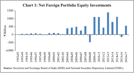
 Increased FPI investments in Indian stock markets have led to their increased participation in the Indian forex market. FPIs participate in the forex market for covering their currency exposures and also for hedging the currency risks in their investment portfolio. The increased FPI activities have facilitated synchronous movements of both markets. The daily movement of USD/INR exchange rates and the equity indices (Sensex and Nifty) during the period 2003-04 to 2016-17 is presented in Chart 2. It shows inverse movements in stock indices and exchange rate, exhibiting a correlation of (-) 0.31 on returns. On the other hand, increased FPI participation in the Indian stock market had a negative effect in terms of rise in volatility in exchange rate and stock indices caused by sudden surge and pause in portfolio flows. During the period 2003-04 to 2007-08, the Indian forex market witnessed a massive surge in capital inflows, resulting in sharp appreciation of the USD/INR exchange rate with the rupee touching a peak of ₹39.20 per US$ on November 7, 2007. The RBI had undertaken large-scale purchases of US$ during this period to curb volatility induced by sharp appreciation of the exchange rate (RBI, 2007). The foreign exchange reserves increased significantly during this period, from US$ 76.1 billion at end-March 2003 to US$ 309.7 billion at end-March 2008. The surplus rupee liquidity on account of large forex purchases by the RBI was sterilised primarily by issuing of government securities and treasury bills under the Market Stabilisation Scheme (MSS). Subsequently, with the collapse of Lehman Brothers, the exchange rate came under massive depreciation pressure and exhibited heightened volatility as the global financial crisis unfolded with full vigour in September 2008. Though the signs of the sub-prime crisis were visible since 2007, it took the shape of a full-blown crisis after the Lehman failure. The large impact of the crisis on the Indian markets was felt from September 2008 to December 2008. During this period, global risk aversion and deleveraging led to capital flows reversal, especially portfolio investments, from the EMEs. India witnessed large FPI sell-off with concomitant pressures on the USD/INR exchange rate (RBI, 2010). The rupee experienced annualised daily volatility of 16.1 per cent from September 2008 to December 2008. It depreciated sharply from around ₹48 per US$ to exceed the then psychological level of ₹50 per US$ on October 24, 2008 (ibid.). The RBI intervened heavily in the foreign exchange market to contain the sharp fall in the rupee by selling about US$ 18.7 billion in the spot market during October 2008 (RBI, 2009). The RBI also took a number of administrative measures, including, among others, the following: provision of a rupee-US dollar swap facility for Indian banks with branches abroad to mitigate their short-term funding pressure; special window to meet the foreign currency requirements of oil marketing companies; measures to encourage capital inflow, viz., increase in interest rate ceiling on FCNR(B) deposits, relaxation of external commercial borrowings guidelines and permitting housing finance companies and NBFCs to raise foreign currency borrowing. The above extraordinary measures by the RBI could calm down the heightened volatility in the forex market by December 2008. The next episode of very high exchange rate volatility was seen during the period after the announcement of tapering off the quantitative easing (famously known as Fed Taper Tantrum) by the US Federal Reserve on May 22, 2013. US bond yields spiked in response to the announcement resulting in narrower interest differentials with respect to EMEs. This led foreign portfolio investors to pull out their investments, especially debt investments, from EMEs including India. The accelerated capital outflows coupled with the prevailing weak macroeconomic situation led to a sharp fall in the rupee by about 19.4 per cent from ₹55.34 per US$ on May 22, 2013 to the historic low of ₹68.85 per US$ on August 28, 2013. The RBI resorted to several monetary and administrative measures to curb the excessive volatility in exchange rates (Pattanaik and Kavediya, 2015). The RBI sold net US$ 10.8 billion in spot during May-August 2013 and also sold heavily in the forward market thus doubling its forward liabilities to US$ 9.1 billion by end-August 2013 (RBI, 2013). It hiked the overnight Marginal Standing Facility (MSF) rate by 200 basis points; limited the overnight injection of liquidity to 0.5 per cent of banks’ net demand and time liabilities; and increased the daily cash reserve maintenance requirement to 99 per cent so as to raise the cost of rupee funding, for banks and non-bank entities, to curb speculative pressure on the rupee. The RBI also took a number of administrative measures such as prohibiting banks to trade in currency futures, curtailing banks’ overnight forex open position limits, restricting import of gold, and opening a concessional swap window for attracting FCNR(B) deposits. The annualised daily volatility of USD/INR exchange rate was at a high of 17 per cent during May 23, 2013 to September 4, 2013. The strong measures taken by the RBI coupled with the forward guidance released by the US Federal Reserve in September 2013 could arrest the heightened volatility in the forex market. The stylised facts described above clearly show the two distinct phases of heightened volatility in the Indian forex market, viz., (a) September to December 2008 - the peak period of the global financial crisis; and (b) May 23, 2013 to September 4, 2013 - the Fed Taper Tantrum period. The comparative descriptive statistics of the daily USD/INR exchange rate returns from April 4, 2005 to March 31, 2017, indicating the two periods of high volatility separately, is provided in Table 1. The daily returns exhibit a wide range of 2.5 to (-)3.0 per cent from September 2008 to December 2008 and 4.0 to (-)1.7 per cent from May 23, 2013 to September 4, 2013. The standard deviation is much higher in both periods compared to the others. | Table 1: Descriptive Statistics of USD/INR Exchange Rate across Different Periods | | Item | Apr 4, 2005 - Aug 31, 2008 | Sep 1, 2008 - Dec 31, 2008 | Jan 1, 2009 - May 22, 2013 | May 23, 2013 - Sep 4, 2013 | Sep 5, 2009 - Mar 31, 2017 | | Mean | 0.0001 | 0.1313 | 0.0129 | 0.2574 | (-)0.0040 | | Maximum | 1.4200 | 2.4900 | 1.9900 | 4.0200 | 1.5500 | | Minimum | (-)1.6200 | (-)3.0100 | (-)2.8200 | (-)1.6900 | (-)2.6800 | | Std. Deviation | 0.33 | 1.02 | 0.56 | 1.08 | 0.38 | | Skewness | 0.14 | (-)0.33 | (-)0.09 | 0.80 | (-)0.81 | | Kurtosis | 5.68 | 3.36 | 4.57 | 4.12 | 9.11 | | Jarque-Bera | 251.96 | 1.83 | 109.54 | 11.66 | 1424.13 | | P-value | <0.01 | 0.40 | <0.01 | <0.01 | <0.01 |
A similar observation can be made from Chart 3 showing these two periods with highly volatile movements in the daily exchange rate returns. There was also a spike in volatility during November-December 2011 due to the Eurozone debt crisis, but it was for a short period. Section IV
Data and Methodology Data The objective of this study is to examine volatility spillovers between the Indian forex and stock markets. Accordingly, we use three variables, viz., daily USD/INR exchange rate return (DER), daily return of S&P BSE Sensex (DSENSEX) and daily return of S&P CNX Nifty (DNIFTY) from April 4, 2005 to March 31, 2017 - a total of 2,899 observations. The continuously compounded daily returns, i.e., DER, DSENSEX, DNIFTY are calculated using the formula Rt = ln(St /St–1) × 100, wherein S is daily spot value of each variable. While the exchange rate refers to the RBI’s reference rate of the Indian rupee per US Dollar obtained from the RBI’s website, the daily closing prices of Sensex and Nifty were obtained from the websites of BSE and National Stock Exchange (NSE), respectively. The SENSEX and NIFTY are the two major equity indices of India and comprise 30 stocks and 50 stocks, respectively. Though both the indices exhibit strong correlation of 0.99, at levels as well as returns, they sometimes exhibit differential movements in terms of returns and volatility because of differences in their composition and sectoral representation of the Indian economy. Therefore, we have used both the indices as a robustness check of our results. As mentioned in Section III, the USD/INR exchange rate volatility heightened during September to December 2008 and from May 23, 2013 to September 4, 2013 with severe impacts and unprecedented regulatory responses. These two periods are well-known for their market-wide impacts, and, therefore, we have taken these two periods separately in this study, similar to the approach followed in Wu (2005), Choi, Fang and Fu (2009), Majumder and Nag (2015), and Xiong and Han (2015)2. The overall sample period is divided into five sub-periods as given in Table 2. Table 3 presents descriptive statistics of all the three variables for the full sample period, which suggest that stock markets are more volatile than the forex market. Average daily returns are positive in both the markets and return distributions are positively skewed. Positive skewness indicates that positive returns are more common than negative returns. Kurtosis, a measure of the magnitude of extremes, is substantially higher than 3 and thus leptokurtic for both stock return as well as exchange rate return. Furthermore, the Jarque–Bera test rejected the null hypothesis of normal distribution for all the variables. All these statistics confirm that returns in both markets are not normally distributed. The descriptive statistics of the sub-samples suggest similar findings, except that the Jarque–Bera test did not reject the null hypothesis of normal distribution in sub-sample II, possibly due to small sample size. | Table 2. Details of the Phases | | Sub-periods | Features | | Period I | Relatively less volatile period (April 4, 2005 to August 31, 2008) | | Period II | Peak of the global financial crisis – Highly volatile period (September 1 to December 31, 2008) | | Period III | Relatively less volatile period (January 1, 2009 to May 22, 2013) | | Period IV | Fed Taper Tantrum- Highly volatile period (May 23 to September 4, 2013) | | Period V | Relatively less volatile period (September 5, 2013 to March 31, 2017) |
| Table 3. Descriptive Statistics | | Item | DER | DSENSEX | DNIFTY | | Mean | 0.01 | 0.05 | 0.05 | | Maximum | 4.02 | 15.99 | 16.33 | | Minimum | -3.01 | -11.60 | -13.01 | | Std. Dev | 0.50 | 1.50 | 1.50 | | Skewness | 0.21 | 0.12 | 0.004 | | Kurtosis | 8.26 | 11.63 | 12.47 | | Jarque-Bera | 3369 (0.00) | 9909 (0.00) | 10842 (0.00) | | LB-Q | 22.6 (0.00) | 24.5 (0.00) | 18.3 (0.00) | | LB-Q2 | 720.1 (0.00) | 443.8 (0.00) | 365.5 (0.00) | | ARCH-LM | 90.6 (0.00) | 62.0 (0.00) | 51.1 (0.00) | | Jarque-Bera (residuals) | 2905 (0.00) | 8246 (0.00) | 10091 (0.00) | DER: USD/INR return; DSENSEX: Sensex return; DNIFTY: Nifty return.
Note: 1. Figures in parentheses are p-values.
2. The statistics provided for Ljung-Box (LB-Q) tests and ARCH langrage multiplier (ARCH-LM) tests have used lag lengths up to 5. | To check stationarity, unit root tests were conducted for all the variables, both for the full sample and all the sub-samples, using Augmented Dicky–Fuller (ADF) and Phillips–Perron (PP) tests. The results confirmed stationarity of all the variables, both in the full sample and all the sub-samples, at 1 per cent level of significance3. The regression is conducted for equation (3) separately for three return variables using ordinary least square, and the Ljung-Box Q-statistics for residuals (LB-Q), squared residuals (LB-Q2) and ARCH langrage multiplier (ARCH-LM) test statistics are reported in Table 3. The rejection of null of serial correlation of squared residuals in LB-Q2 and ARCH-LM tests and the rejection of normality in the Jarque–Bera test validate the use of ARCH type of models to study the dynamic interdependence of the variables. Methodology The dynamic linkages between stock market and foreign exchange market are examined in terms of the conditional second moments of their distributions, termed as volatility spillover. We specify and estimate a multivariate model using daily data on stock and exchange rate returns that allows the possibilities of different types and categories of news simultaneously affecting the conditional variances. Before proceeding to estimate volatility spillovers, we employ Granger causality tests (Granger, 1969) to examine the possible endogeneity between these variables4. This section describes the specific model employed to examine the spillovers and its econometric properties as well as the estimation strategy. Granger Causality Test The Granger causality test involves estimating the following pairs of equations in a vector autoregression (VAR) framework:
Multivariate GARCH (MGARCH) A standard VAR is suitable where the residual vector is assumed to be a white noise process with time invariant covariance matrix. However, returns on financial assets typically exhibit ‘volatility clustering’ which strongly suggests the need for modelling time-varying second-order moments, popularly known as Autogressive Conditional Heteroskedasticity (ARCH). A variant of ARCH, i.e., Generalised Autogressive Conditional Heteroskedasticity (GARCH) models are developed to consider time varying second order moments. MGARCH models and their extensions are widely used to examine the relationship between two or more financial variables/financial market volatility in the presence of endogeneity. We estimate a variant of MGARCH model, which also takes into account the asymmetric specifications of Nelson (1991) and the multivariate extension proposed by Kroner and Ng (1998). The bivariate version of the MGARCH model is used to examine spillovers across two markets as proposed by Engle and Kroner (1995), i.e., a bivariate BEKK-GARCH (1,1) model, where the system of conditional mean equations consists of VAR(p) models (p = 1, ..., n). The specification for conditional mean equation in VAR(p) form is: The conditional variance equation is expressed in terms of BEKK specification, which ensures positive semi-definiteness of the conditional variance matrix and is less cumbersome to estimate, with the advantage of estimating less number of parameters: To incorporate asymmetric responses of volatility in the variances and covariances, the above model can be further extended as proposed by Kroner and Ng (1998): 
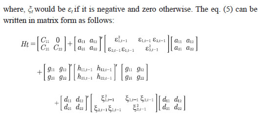 In the above model, the off-diagonal parameters in matrices A and G measure volatility spillover between markets while the diagonal parameters in those matrices capture the effects of their own past shocks and volatility. The diagonal parameters in matrix D measure the response to own past negative shocks while the off-diagonal parameters dij show the response of one market to negative shocks in the other market, to be called hereafter as cross-market asymmetric responses. A negative value of D means negative news tend to increase volatility more than the positive news. In case of exchange rate, Nath and Pacheco (2018) define that a negative value of the coefficient implies that a negative shock (the appreciation of the rupee) increases volatility in forex market more than positive shock (the depreciation of the rupee) and a positive value of the coefficient implies that a positive shock (depreciation of the rupee) increases volatility more than the negative shock (appreciation of the rupee). The above BEKK model can be estimated efficiently and consistently using full information maximum-likelihood method (Engle and Kroner, 1995; Kroner and Ng, 1998). The log-likelihood function assuming normally distributed errors can be stated as: 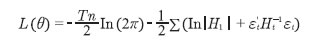 where T is the number of observations, n is the number equations and θ represents the parameter vector to be estimated. To obtain the estimates of the parameters, a combination of the standard gradient search algorithm Broyden– Fletcher–Goldfarb–Shanno (BFGS) and simplex algorithm is used. Section V
Empirical Analysis Test for Causality We examined the causal relationship between exchange rate return and stock index return by applying the Granger causality test. The test is conducted using 3 lags based on Schwartz criteria and the results are reported in Table 4. The results show that the F-statistics is significant at less than 5 per cent level in all the cases. Thus, the null of stock return (exchange rate return) does not cause exchange rate return (stock return) is rejected; hence suggesting the presence of bidirectional causality between stock returns and exchange rate returns in India. This indicates the presence of endogeneity between the two variables. Therefore, any type of univariate models to study volatility spillovers may provide biased results. Hence, we used MGARCH model in this study. Bivariate BEKK-GARCH (1,1) Estimation Results It is commonly observed that the financial markets exhibit asymmetric effects. Following Apte (2001), Yang and Doong (2004), Wu (2005), Majumder and Nag (2015), and Behera (2017), we tried to capture asymmetric effects in our model. We have estimated the model for both full sample and five sub-samples. The preferred lag lengths for the full sample and all sub-samples are based on Hosking’s multivariate Q-test. The estimation is conducted using two groups of variables: (i) DER and DSENSEX and (ii) DER and DNIFTY. The estimates of bivariate asymmetric GARCH(1,1)-BEKK parameters along with various diagnostic test results are reported in Tables 5 through 8. The results for the conditional mean equation and conditional variance equation are reported separately. | Table 4. Granger Causality Test Results | | Null Hypothesis | F-Statistics | P-value | | DSENSEX does not granger cause DER | 48.23 | 0.00 | | DER does not granger cause DSENSEX | 3.11 | 0.03 | | DNIFTY does not granger cause DER | 49.67 | 0.00 | | DER does not granger cause DNIFTY | 3.42 | 0.02 | The results of conditional mean equations in Tables 5 and 6 indicate that the autoregressive coefficients are statistically significant in the case of DER for the full sample and sub-samples 2 and 3, and also in the case of DSENSEX and DNIFTY for the full sample and sub-samples 1 and 5. This establishes that exchange rate returns as well as stock market returns largely depend on their own past values. The off-diagonal parameter (γ21) is found to be statistically significant in the full sample and all sub-samples except for sub-sample 4. However, the γ12 coefficient is statistically insignificant in most cases except in sub-sample 5, when DNIFTY is used as a measure of stock return. The results indicate that stock markets do have price spillover effects on the foreign exchange market, but not the vice-versa. Further, the negative value of the coefficients indicate negative relationship, i.e., rise in stock price (positive stock returns) leads to appreciation in USD/INR exchange rate (negative exchange rate return) and vice-versa. The main focus of our study is to analyse volatility transmission between forex and stock markets, which can be inferred from the estimated parameters in the conditional variance equations. The results relating to conditional variance equations are provided in Tables 7 and 8. In both the conditional variance equations, the estimated diagonal parameters a11 (full sample and all sub-samples except sub-sample 2), a22 (full sample and sub-sample 3), g11 (full sample and all sub-samples except sub-sample 4) and g22 (full sample and all sub-samples) are statistically significant, indicating a strong GARCH(1,1) process, which establishes that volatility in stock and forex markets is driven by their own past shocks and volatility. The large magnitudes of g11 and g22 indicate strong volatility persistence. The coefficient g11 is found to be insignificant in sub-sample 4, suggesting that exchange rate volatility was not persistent during that period. The a12 is statistically significant in 2nd, 4th and 5th sub-samples in the case of DSENSEX and in 4th and 5th sub-samples in the case of DNIFTY, indicating shock spillover from forex market to stock markets mainly during the high volatile periods, i.e., 2nd and 4th sub-samples. The coeffecient g12 is statistically significant in the 2nd sub-sample in the case of DSENSEX and in the 1st and 2nd sub-samples in the case of DNIFTY. The results establish the existence of volatility spillovers from the forex market to stock markets mainly during the 2nd sub-sample period - the peak of the global financial crisis. We did not find shock/volatility spillovers from forex market to stock markets in the full sample period. The volatility spillovers from forex market to stock market during highly volatile periods is possibly due to presence of many export oriented heavy weight companies like Infosys, TCS, Wipro, and Sun Pharma in the Sensex/Nifty indices which are highly sensitive to exchange rate movements. | Table 5. Estimated Asymmetric MGARCH-BEKK Model - Mean Equation (Sensex) | | Variables | Full Sample
(Apr. 1, 2005 to Mar. 31, 2017) | Sub-Sample 1
(Apr. 1, 2005 to Aug. 31, 2008) | Sub-Sample 2
(Sept. 1, 2008 to Dec. 31, 2008) | Sub-Sample 3
(Jan. 1, 2009 to May 22, 2013) | Sub-Sample 4
(May 23, 2013 to Sept. 4, 2013) | Sub-Sample 5
(Sept. 5, 2013 to Mar. 31, 2017) | | Dependent Variable: DER | | DERt-1 | -0.04 | -(1.95)** | -0.01 | -(0.23) | -0.19 | -(1.87)* | -0.07 | -(2.31)** | -0.17 | -(1.48) | -0.06 | -(1.40) | | DERt-2 | -0.04 | -(2.39)** | | | | | | | | | -0.02 | -(0.51) | | DSENSEXt-1 | -0.04 | -(8.65)*** | -0.03 | -(4.87)*** | -0.12 | -(4.09)*** | -0.09 | -(7.46)*** | -0.11 | -(1.13) | -0.06 | -(4.13)*** | | DSENSEXt-2 | -0.01 | -(1.53) | | | | | | | | | 0.003 | (0.22) | | Constant | 0.01 | (1.02) | 0.003 | (0.39) | 0.11 | (1.08) | 0.01 | (0.61) | 0.20 | (1.92)* | 0.01 | (0.48) | | | Dependent Variable: DSENSEX | | DERt-1 | -0.05 | -(1.16) | -0.05 | -(0.39) | -0.14 | -(0.40) | 0.01 | (0.12) | 0.24 | (1.50) | -0.15 | -(1.42) | | DERt-2 | -0.02 | -(0.49) | | | | | | | | | 0.06 | (0.61) | | DSENSEXt-1 | 0.05 | (2.64)*** | 0.10 | (2.95)*** | 0.02 | (0.14) | 0.02 | (0.87) | 0.08 | (0.69) | 0.08 | (1.91)* | | DSENSEXt-2 | -0.03 | -(1.43) | | | | | | | | | -0.06 | -(1.34) | | Constant | 0.05 | (2.80)*** | 0.12 | (2.87)*** | -0.46 | -(1.29) | 0.03 | (1.02) | -0.19 | -(1.30) | 0.04 | (1.30) | *,*,***: Indicates significant at 10 per cent, 5 per cent and 1per cent levels, respectively.
Note: Figures in parentheses are t-statistics. |
| Table 6. Estimated Asymmetric MGARCH-BEKK Model - Mean Equation (Nifty) | | Variables | Full Sample
(Apr. 1, 2005 to Mar. 31, 2017) | Sub-Sample 1
(Apr. 1, 2005 to Aug. 31, 2008) | Sub-Sample 2
(Sept. 1, 2008 to Dec. 31, 2008) | Sub-Sample 3
(Jan. 1, 2009 to May 22, 2013) | Sub-Sample 4
(May 23, 2013 to Sept. 4, 2013) | Sub-Sample 5
(Sept. 5, 2013 to Mar. 31, 2017) | | Dependent Variable: DER | | DERt-1 | -0.04 | -(2.05)** | -0.01 | -(0.32) | -0.19 | -(1.85)* | -0.08 | -(2.65)*** | -0.17 | -(1.54) | -0.06 | -(1.37) | | DERt-2 | -0.04 | -(2.61)*** | | | | | -0.05 | -(1.97)** | | | | | | DNIFTYt-1 | -0.04 | -(10.10)*** | -0.03 | -(4.79)*** | -0.13 | -(3.94)*** | -0.09 | -(7.61)*** | -0.12 | -(1.31) | -0.06 | -(4.36)*** | | DNIFTYt-2 | -0.01 | -(1.75)* | | | | | -0.02 | -(1.46) | | | | | | Constant | 0.005 | (0.97) | 0.002 | (0.30) | 0.12 | (1.18) | 0.01 | (0.64) | 0.19 | (1.92)* | 0.01 | (0.61) | | | Dependent Variable: DNIFTY | | DERt-1 | -0.06 | -(1.49) | -0.08 | -(0.52) | -0.15 | -(0.43) | 0.03 | (0.51) | 0.24 | (1.53) | -0.18 | -(1.75)* | | DERt-2 | -0.02 | -(0.37) | | | | | 0.05 | (0.99) | | | | | | DNIFTYt-1 | 0.04 | (2.29)** | 0.10 | (2.79)*** | 0.03 | (0.25) | 0.03 | (0.94) | 0.08 | (0.78) | 0.07 | (1.82)* | | DNIFTYt-2 | -0.02 | -(1.18) | | | | | 0.04 | (1.29) | | | | | | Constant | 0.05 | (2.90)*** | 0.12 | (2.68)*** | -0.43 | -(1.30) | 0.03 | (0.91) | -0.25 | -(1.70)* | 0.04 | (1.36) | *,*,***: Indicates significant at 10 per cent, 5 per cent and 1 per cent levels, respectively.
Note: Figures in parentheses are t-statistics. |
| Table 7. Estimated Asymmetric MGARCH-BEKK Model - Variance Equation (Sensex) | | Coefficients | Full Sample
(Apr. 1, 2005 to Mar. 31, 2017) | Sub-Sample 1
(Apr. 1, 2005 to Aug. 31, 2008) | Sub-Sample 2
(Sept. 1, 2008 to Dec. 31, 2008) | Sub-Sample 3
(Jan. 1, 2009 to May 22, 2013) | Sub-Sample 4
(May 23, 2013 to Sept. 4, 2013) | Sub-Sample 5
(Sept. 5, 2013 to Mar. 31, 2017) | | a11 | 0.35 | (16.85)*** | 0.51 | (13.09)*** | -0.13 | (1.58) | 0.33 | (6.78)*** | -0.39 | -(2.26)** | 0.22 | (3.92)*** | | a12 | -0.04 | -(0.83) | 0.08 | (0.45) | -0.70 | -(1.75)* | 0.01 | (0.26) | 0.66 | (2.96)*** | -0.26 | -(2.12)** | | a21 | -0.01 | -(1.28) | 0.02 | (1.87)* | 0.01 | (0.17) | -0.01 | -(0.82) | -0.14 | -(0.94) | 0.01 | (0.86) | | a22 | 0.15 | (7.13)*** | -0.01 | -(0.17) | 0.03 | (0.24) | 0.12 | (3.39)**** | 0.23 | (1.51) | -0.06 | -(0.78) | | g11 | 0.93 | (123.80)*** | 0.84 | (35.23)*** | 0.84 | (7.75)*** | 0.92 | (34.11)*** | 0.19 | (0.79) | 0.96 | (54.67)*** | | g12 | -0.001 | -(0.17) | -0.13 | -(1.30) | -1.21 | -(2.48)** | -0.01 | -(0.28) | -0.28 | -(1.09) | 0.03 | (0.72) | | g21 | 0.001 | (0.82) | 0.002 | (0.60) | 0.08 | (2.88)*** | -0.01 | -(1.40) | -0.38 | -(2.75)*** | 0.001 | (0.13) | | g22 | 0.95 | (158.91)*** | 0.86 | (44.55)*** | 0.72 | (10.52)**** | 0.98 | (160.43)*** | 0.67 | (4.52)**** | 0.94 | (50.66)*** | | d11 | -0.06 | -(1.41) | -0.08 | (0.66) | -0.04 | -(0.26) | -0.04 | -(0.51) | -0.05 | -(0.18) | 0.08 | (1.00) | | d12 | 0.02 | (0.23) | -0.03 | -(0.11) | -0.04 | -(0.05) | -0.06 | -(0.76) | -0.04 | -(0.06) | 0.10 | (0.79) | | d21 | -0.01 | -(1.79)* | 0.04 | (4.73)*** | 0.18 | (3.63)*** | 0.01 | (0.61) | 0.72 | (3.85)*** | -0.04 | -(1.66)* | | d22 | 0.33 | (12.35)*** | -0.61 | -(11.19)*** | -0.51 | -(2.10)** | 0.24 | (7.00)*** | 0.25 | (1.32) | 0.33 | (6.27)*** | | N | 2897 | | 834 | | 76 | | 1057 | | 72 | | 854 | | | Log-likelihood | -6000 | | -1579 | | -295 | | -2441 | | -211 | | -1329 | | *,*,***: Indicates significant at 10 per cent, 5 per cent and 1per cent levels, respectively.
Note: 1. Figures in parentheses are t-statistics.
2. Subscripts 1 and 2 of each parameter represent forex and stock markets, respectively. |
| Table 8. Estimated Asymmetric MGARCH-BEKK Model - Variance Equation (Nifty) | | Coefficients | Full Sample
(Apr. 1, 2005 to Mar. 31, 2017) | Sub-Sample 1
(Apr. 1, 2005 to Aug. 31, 2008) | Sub-Sample 2
(Sept. 1, 2008 to Dec. 31, 2008) | Sub-Sample 3
(Jan. 1, 2009 to May 22, 2013) | Sub-Sample 4
(May 23, 2013 to Sept. 4, 2013) | Sub-Sample 5
(Sept. 5, 2013 to Mar. 31, 2017) | | a11 | 0.35 | (16.28)*** | 0.52 | (13.31)*** | -0.13 | -(1.00) | 0.34 | (6.83)*** | 0.39 | (2.19)** | 0.20 | (3.66)*** | | a12 | -0.04 | -(0.89) | 0.12 | (0.75) | -0.63 | -(1.58) | 0.001 | (0.01) | -0.70 | -(3.06)*** | -0.26 | -(1.74)* | | a21 | -0.01 | -(1.22) | 0.02 | (2.39)** | 0.01 | (0.24) | -0.01 | -(0.56) | 0.12 | (0.86) | 0.01 | (1.03) | | a22 | 0.16 | (7.60)*** | -0.02 | -(0.39) | 0.05 | (0.35) | 0.12 | (4.28)*** | -0.22 | -(1.50) | -0.05 | -(0.62) | | g11 | 0.93 | (119.49)*** | 0.84 | (36.53)*** | 0.83 | (7.51)*** | 0.91 | (32.88)*** | 0.20 | (0.78) | 0.97 | (57.91)*** | | g12 | -0.001 | -(0.08) | -0.15 | -(2.05)** | -1.22 | -(2.70)*** | -0.004 | -(0.18) | -0.28 | -(1.03) | 0.01 | (0.30) | | g21 | 0.001 | (0.82) | -0.00001 | -(0.003) | 0.09 | (3.22)*** | -0.009 | -(1.80) | -0.35 | -(2.52)** | 0.01 | (0.72) | | g22 | 0.95 | (155.01)*** | 0.84 | (39.91)*** | 0.72 | (9.33)*** | 0.98 | (137.9)*** | 0.68 | (4.25)*** | 0.92 | (41.89)*** | | d11 | -0.07 | -(2.10)** | 0.02 | (0.17) | 0.04 | (0.22) | -0.05 | -(0.61) | -0.05 | -(0.21) | -0.07 | -(0.75) | | d12 | 0.02 | (0.24) | 0.03 | (0.08) | 0.18 | (0.24) | -0.05 | -(0.61) | -0.06 | -(0.11) | -0.13 | -(0.90) | | d21 | -0.01 | -(1.71)* | -0.03 | -(3.73)*** | -0.19 | -(3.51)*** | 0.02 | (0.87) | 0.68 | (3.86)*** | 0.05 | (2.35)** | | d22 | 0.33 | (12.28)*** | 0.64 | (11.18)*** | 0.48 | (1.88)* | 0.26 | (6.72)*** | 0.22 | (1.09) | -0.36 | -(6.75)*** | | N | 2897 | | 834 | | 76 | | 1056 | | 72 | | 855 | | | Log-likelihood | -6029 | | -1587 | | -292 | | -2446 | | -213 | | -1340 | | *,*,***: Indicates significant at 10 per cent, 5 per cent and 1 per cent levels, respectively.
Note: 1. Figures in parentheses are t-statistics.
2. Subscripts 1 and 2 of each parameter represent forex and stock markets, respectively | In both DSENSEX and DNIFTY, the a21 is found to be significant in 1st sub-sample, whereas g21 is found to be significant in both 2nd and 4th sub-samples. We did not find shock/volatility spillovers from stock market to forex market when the full sample period was considered. The results suggest that the volatility spillover from stock market to the forex market was restricted to the high exchange rate volatility periods, viz., 2nd and 4th sub-samples. Unlike the price spillovers from stock market to forex market, which was found to be a common phenomenon across the full sample period, the volatility spillovers from stock market to forex market was more of a specific phenomenon observed only during the high exchange rate volatility periods. The asymmetry parameter d12 is not statistically significant in respect of both DSENSEX and DNIFTY. The parameter d21 is found significant for the full sample as well as all sub-samples except for the 3rd sub-sample in respect of both DSENSEX and DNIFTY. These findings confirm asymmetric responses of the foreign exchange market to negative shocks in stock markets in the full sample period. Section VI
Conclusion The bivariate BEKK-GARCH analysis suggests that there is one way price spillovers from stock markets to forex market in India. This implies the dominance of the portfolio channel in the price relationship between the exchange rate and stock prices in India. The volatilities in both the markets are found to be highly persistent and are driven by their own past shocks and volatility. With regard to volatility spillovers, unlike the price spillovers, we did not find any volatility spillover effects between these two markets when the full sample period was considered. The volatility spillovers were found to be more of a specific phenomenon, observed mainly during the periods of high exchange rate volatility. The volatility spillovers from stock markets to the forex market were evident during the 2nd and 4th sub-sample periods, while that from the forex market to stock market was observed mainly during the 2nd sub-sample period. The 2nd and 4th sub-sample periods represent the onset of the global financial crisis and the Fed Taper Tantrum, respectively-marked as heightened volatility periods. The results also establish asymmetric responses of the forex market to negative shocks in the stock market. The findings justify our approach of conducting sub-period analysis. The evidence of volatility spillovers between both the markets during highly volatile periods points to the possible ‘contagion’ impact, apart from the volatility transmission caused by the large FPI investment/disinvestment actions. This observation is in line with the evidence provided by King and Wadhwani (1990) regarding the existence of high contagion effects during volatile market conditions in their study on transmission of volatility between stock markets. The market contagion amplifies volatility and exacerbates stress in the financial system as a whole. The findings of this paper may help financial sector regulators to devise appropriate policies and strategies to proactively deal with the volatility spillover effects when the USD/INR exchange rate exhibits high volatility. These findings may also help international investors and portfolio managers to formulate suitable trading/hedging/portfolio diversification strategies to deal with the impact of volatility spillovers during stressful market conditions.
References Abdalla, I.S.A., and V. Murinde (1997). ‘Exchange rate and stock price interactions in emerging markets: Evidence on India, Korea, Pakistan and the Philippines’, Applied Financial Economics, 7(1): 25–35. Agénor, P. (2003). ‘Benefits and costs of international financial integration: Theory and facts’. The World Economy, 26(8): 1089–1118. Ajayi, R. A., J. Friedman and S. M. Mehdian (1998). ‘On the relationship between stock returns and exchange rates: Tests of Granger causality’, Global Finance Journal, 9(2): 241–51. Alaganar, V. T. and R. Bhar (2007). ‘Empirical properties of currency risk in country index portfolios’, The Quarterly Review of Economics and Finance, 47:159–74. Aloui, C. (2007). ‘Price and volatility spillovers between exchange rates and stock indexes for the pre- and post-euro period’, Quantitative Finance, 7(6): 1–17. Apte, P. (2001). ‘The interrelationship between stock markets and the foreign exchange market’, Prajnan, 30: 17–29. Assoe, K. (2001). ‘Volatility spillovers between foreign exchange and emerging stock markets’, CETAI, Cahiers de recherché, 2001-04. Aydemir, O., and E, Demirhan. (2009). ‘The relationship between stock prices and exchange rates: Evidence from Turkey’, International Research Journal of Finance and Economics, 23(2): 207–15. Bahmani-Oskooee, M. and A. Sohrabian. (1992). ‘Stock prices and the effective exchange rate of the dollar’, Applied Economics, 24(4): 459–64. Behera, H. (2017). ‘Spillover effects of foreign institutional investments in India’, International Journal of Bonds and Derivatives, 3(2): 132–52. Bonga-Bonga, L., and J. Hoveni (2011). ‘Volatility spillover between the equity market and foreign exchange market in South Africa’, Working Paper 252, University of Johannesburg. Chang H. L., C. W. Su and Y. C. Lai (2009). ‘Asymmetric price transmissions between the exchange rate and stock market in Vietnam’, International Research Journal of Finance and Economics, 23: 104–13. Choi, D. F. S., V. Fang and T. Y. Fu (2009). ‘Volatility spillovers between New Zealand stock market returns and exchange rate changes before and after the 1997 Asian financial crisis”, Asian Journal of Finance and Accounting, 1(2): 107–17. Cournot, A. (1927). Researches into the mathematical principles of the theory of wealth, trans. Nathaniel T. Bacon, New York: Macmillan. Dornbusch, R. and S. Fisher (1980). ‘Exchange rates and the current account’, American Economic Review, 70: 960–71. Engle, R. F., and K. F. Kroner (1995). ‘Multivariate simultaneous generalized ARCH’, Econometric Theory, 11: 122–50. Eun, C. S., and B. G. Resnick (1988). ‘Exchange rate uncertainty, forward contracts, and international portfolio selection’, Journal of Finance, 43: 197– 215. Fedorova, E. and K. Saleem (2010). ‘Volatility spillovers between stock and currency markets: Evidence from emerging Eastern Europe’, Finance a úvěr- Czech Journal of Economics and Finance, 60(6), 519-533. Frankel, J. A. (1983). ‘Monetary and portfolio-balance models of exchange rate determination’, in Economic Interdependence and Flexible Exchange Rates, ed. J. Bhandari and B. Putnam, Cambridge, MA: MIT Press, pp 84–114. Gavin, M. (1989). ‘The stock market and exchange rate dynamics’, Journal of International Money and Finance, 8(2): 181–200. Granger, C. W. (1969). ‘Investigating causal relations by econometric models and cross-spectral methods’, Econometrica, 37: 424–39. Granger, C. W., B. N. Huangb and C. W. Yang (2000). ‘A bivariate causality between stock prices and exchange rates: Evidence from recent Asianflu’, The Quarterly Review of Economics and Finance, 40(3): 337–54. Huzaimi, H., and V. K. Liew (2004). ‘Causal relationships between exchange rate and stock prices in Malaysia and Thailand during the 1997 currency crisis turmoil’. Available at: http://129.3.20.41/eps/if/papers/0405/0405015.pdf. Issam S. A. Abdalla and V. Murinde (1997). ‘Exchange rate and stock price interactions in emerging financial markets: Evidence on India, Korea, Pakistan and the Philippines’, Applied Financial Economics, 7(1): 25–35. Ito, T. and W-L. Lin (1994). ‘Price volatility and volume spillovers between the Tokyo and New York Stock Markets’, in The internationalization of equity markets, ed. J. A. Frankel, University of Chicago Press, Chicago, pp. 309–343. Jebran, K. and A. Iqbal (2016). ‘Dynamics of volatility spillover between stock market and foreign exchange market: Evidence from Asian Countries’, Financial Innovation, 2(3): 1-20. Kanas, A. (2000). ‘Volatility spillovers between stock returns and exchange rate changes: International evidence’, Journal of Business Finance and Accounting, 27(3&4): 447–67. King, M. and S. Wadhwani (1990). ‘Transmission of volatility between stock markets’, The Review of Financial Studies, 3(1): 5–33. Kisaka, S. E., and A. Mwasaru (2012). ‘The causal relationship between exchange rates and stock prices in Kenya’, Research Journal of Finance and Accounting, 3(7): 121-131. Kose, Y., M. Doganay and H. Karabacak (2010). ‘On the causality between stock prices and exchange rates: Evidence from Turkish financial market’, Problems and Perspectives in Management, 8(1):127-135. Kroner, K., and V. Ng (1998). ‘Modelling asymmetric comovements of asset returns’, The Review of Financial Studies, 11(4): 817–44. Majumder, S. B., and R.N. Nag (2015). ‘Return and volatility spillover between stock price and exchange rate: Indian evidence’, International Journal of Economics and Business Research, 10(4): 326-340. Mishra, A. K. (2004). “Stock Market and Foreign Exchange Market in India: Are they Related?”, South Asia Economic Journal, 5(2): 209-232. Mishra, A. K., N. Swain and D. K. Malhotra (2007). ‘Volatility spillovers between stock and foreign exchange markets: Indian evidence’, International Journal of Business, 12(3): 344–59. Mitra, P. K. (2017). ‘Dynamics of volatility spillover between the Indian stock market and foreign exchange market return’, Academy of Accounting and Finance Studies Journal, 21(2): 1-12. Mok, H. M. (1993). ‘Causality of interest rate, exchange rate and stock prices at stock market open and close in Hong Kong’, Asia Pacific Journal of Management, 10(2): 123–43. Morales, L. (2008). ‘Volatility spillovers between equity and currency markets: Evidence from major Latin American countries’, Cuadernos de Economica, Latin American Journal of Economics, 45 (November): 185–215. Nath, G. and G. P. Samanta (2003). ‘Integration between Forex and Capital Markets in India: An EmpiricalExploration’,Available at: https://ssrn.com/abstract=475822. Nath, G. and M. Pacheco (2018). ‘Currency futures market in India: An empirical analysis of market efficiency and volatility’, Macroeconomics and Finance in Emerging Market Economies, 11(1): 47–84. Nelson, D. B. (1991). ‘Conditional heteroskedasticity in asset returns: A new approach’, Econometrica, 59(2): 347–70. Pattanaik, S., and R. Kavediya (2015). ‘Taper talk impact on the rupee: Preconditions for the success of an interest rate defence of the exchange rate’, Prajnan, XLIV(3): 251-277. Pan, M. S., R. C. W. Fok and Y. A. Liu (2007). ‘Dynamic linkages between exchange rates and stock prices: Evidence from East Asian markets’, International Review of Economics & Finance, 16(4): 503–20. Panda, P. and M. Deo (2014). ‘Asymmetric and volatility spillover between stock market and foreign exchange market: Indian experience’, The IUP Journal of Applied Finance, 20(4): 69-82. Phylaktis, K. and F. Ravazzolo. 2002. ‘Stock prices and exchange rate dynamics’, Cass Business School Working Paper. Pradhan, C. P. (2006). ‘The dynamic relationship between the stock price and exchange rate in India’, The IUP Journal of Monetary Economics, IV: 26–36. Rahman, M. L., and J. Uddin (2009). ‘Dynamic relationship between stock prices and exchange rates: Evidence from three South Asian countries’, International Business Research, 2(2): 167–74. Reserve Bank of India (2007). Report on Currency and Finance 2005–06, 31 May. — (2009). Annual Report 2008–09, 27 August. — (2010). Report on Currency and Finance 2008–09, 1 July. — (2013). Reserve Bank of India Bulletin – October 2013, 10 October. Rubayat, S. and M. Tereq (2017). ‘Volatility spillover between foreign exchange market and stock market in Bangladesh’, 11th International Conference on Management Science and Engineering Management, June. Smyth, R., and M. Nandha (2003). ‘Bivariate causality between exchange rates and stock prices in South Asia’, Applied Economics Letters, 10(11): 699–704. Wu, R. (2005). ‘International transmission effect of volatility between the financial markets during the Asian financial crises’, Transition Studies Review, 12(1): 19–35. Xiong, Z. and L. Han (2015). ‘Volatility spillover effect between financial markets: Evidence since the reform of the RMB exchange rate mechanism’, Financial Innovation (a Springer Open Journal),1(9):1-12. Yang, S. and S. Doong (2004). ‘Price and volatility spillovers between stock prices and exchange rates: Empirical evidence from the G-7 countries’, International Journal of Business and Economics, 3(2): 139–53.
|