|
Abstract
This study provides the context, rationale and analytical framework of the finance-neutral output gap (FNOG) of an economy. In the conventional (inflation-neutral) output gap measure, inflation is the sole indicator of the state of the economy; in other words, imbalances in the economy are reflected solely in high or low inflation in this measure. However, in the FNOG, heightened levels of financial variables in the form of excessive credit growth and unsustainable asset market returns are the key sources of imbalances rather than inflation. A comparison of the conventional output gap versus FNOG in the Indian context suggests significant divergence between the two. Latest data suggest that the FNOG in India has closed in recent quarters faster than the conventional output gap due to an acceleration in credit growth and buoyant asset market conditions.
I. Introduction
The output gap represents the deviation of actual output from the “potential” output, the latter defined as the maximum level of economic activity that an economy can achieve when operating at full capacity. The output gap can be positive or negative and it is reflective of the cyclical position of the economy. A positive output gap, which results when actual output is above potential output, reflects excess demand in the economy which can generate inflationary pressures. In contrast, a negative output gap – actual output being lower than potential output – occurs when the available resources in the economy are not fully utilised and reflects deficient demand.
The output gap, being a summary measure of demand conditions in the economy, provides a useful indicator of the state of the macro economy and is used as an important input for monetary policy. Conventionally, inflation has been seen as the sole symptom of macroeconomic imbalances in the economy, captured by fluctuations in various measures of the output gap. However, there have been instances in history, when inflation was low and stable, even as output was expanding unsustainably.
A case in point was a massive build-up of financial imbalances as reflected in excessive credit growth and high asset prices before the global financial crisis (GFC) hit in August 2008. Large credit growth fuelled demand for housing and other assets, driving up their prices and increasing incomes of both households and firms. This encouraged banks further to extend credit for financing more investment. Economic expansion resulting from new capacity additions itself eased the supply constraints and led to an increase in the overall growth in many economies. Further, this strong financial boom resulted in large capital flows to emerging market economies, leading to appreciation of their currencies. These factors exerted downward pressure on prices keeping inflation benign. Going by conventional wisdom one could interpret that such high economic growth coupled with benign inflation was sustainable. However, a closer look at financial sector data revealed that this rapid economic growth spurred by the financial boom, resulted in large misallocation of resources and unsustainable asset prices. Once the crisis hit and financial conditions turned tight, aggregate demand worsened and many of these economies eventually plunged into a prolonged recessionary phase.
The above referred developments led to a new measure of output gap, popularly known as the finance-neutral output gap or FNOG (Borio et al., 2013), which evaluates the sustainability of economic growth based on financial developments captured by movements in bank credit and asset markets, rather than inflation. In this measure, the positive output gap reflects overheating in the economy due to excessive financial market activities, while negative output gap reflects the existence of a slack in the economy due to depressed financial conditions. Leading central banks, including the Bank of England, the European Central Bank, Banco de Espan᷉a, etc., use the FNOG as one of the inputs for monetary policy. International organisations such as the International Monetary Fund (IMF), the Bank for International Settlements (BIS) and the Asian Development Bank (ADB) have also emphasised the usefulness of the FNOG for monetary policy.
The FNOG has also been estimated in the Indian context (Rath et al., 2017). This estimate is now incorporated along with conventional measures of the output gap by the Reserve Bank in its Monetary Policy Report since October 2017. The methodology for estimating the FNOG and the empirical estimates in the Indian context are explained below. The technical details are in the Annex.
II. Conventional Output Gap and FNOG - Measurement
Unlike actual output, the level of potential output and, hence, the output gap cannot be observed directly and is estimated from the other available macroeconomic data. Various methodologies have been used to estimate potential output, but they all assume that output can be divided into a trend (a measure of potential output) and a cyclical component (a measure of the output gap).
The most common statistical approach to estimate potential output and output gap is the use of univariate statistical filters such as, Hodrick-Prescott (HP) filter, which help extract the cycle (output gap) and trend (potential output) from the observed output data (Annex). The advantage of the univariate approach is that it is simple and can be applied directly to the output data, i.e., gross domestic product (GDP).
However, output gap estimates from the univariate filters have several limitations. They are purely statistical in nature and do not incorporate any economic structure and hence may not be consistent with any economic concept of potential output or output gap. Further, univariate statistical filters typically suffer from end-point problem, whereby the latest estimates of trend and cycle undergo large revisions with the arrival of new information. Hence, they may provide less precise estimates for the latest period, which matters most for policy making.
To overcome the above referred problems associated with univariate approaches, a Multi-Variate Kalman Filter (MVKF) technique is followed that allows exploitation of other macroeconomic data, which are observable. For measuring conventional output gap using MVKF, researchers have typically included inflation as an additional variable as it is considered as the sole source of unsustainability. The output gap, thus obtained, is called the inflation-neutral output gap. In the FNOG measured with the MVKF, researchers have used a set of financial variables instead of inflation. Financial variables used are mainly real bank credit growth and real stock market return (Annex). Thus, as against the inflation-neutral measure, which incorporates inflation as the source of unsustainability, in the FNOG, financial variables are used for estimating the output gap (Annex).
III. Empirical Estimates of FNOG for India
Following the methodology explained in the previous section, the FNOG was estimated for India and compared with the conventional output gap measures. The study is based on GDP data from Q1:2006-07 to Q3:2017-18. As the back series of GDP (Base 2011-12) is not yet available, it was obtained by applying the technique of splicing2.
For measuring the FNOG, the real policy repo rate, real bank credit growth and real stock market return were used as the explanatory variables. This real policy rate was represented by the policy repo rate, deflated with one period ahead (realised) consumer price index (CPI) inflation. Bank credit growth and stock market return were measured using the seasonally adjusted quarterly changes in the non-food credit of scheduled commercial banks (SCBs) and the BSE Sensex respectively, deflated by CPI inflation3.
The estimated results, presented in Table 1, suggest that the real policy rate affects the FNOG negatively with a lag of four quarters. Real credit growth and real stock market return affect the FNOG positively with a lag of two quarters and one quarter, respectively.
| Table 1: Regression Estimates - Dependent Variable: Output Gap (yt) |
| Independent Variables |
Coefficient |
Standard Error |
p-value |
| yt-1 |
0.04 |
0.24 |
0.87 |
| rt-4 |
-0.25** |
0.14 |
0.08 |
| bct-2 |
0.17** |
0.09 |
0.07 |
| sensext-1 |
0.06* |
0.02 |
0.01 |
Note: ** Significant at 5 per cent; * Significant at 10 per cent.
yt : Output gap; rt: real interest rate; bct: real bank credit growth; sensext: real BSE sensex returns
Source: Database on Indian Economy (DBIE), RBI and authors’ calculations. |
A time plot of FNOG estimates in Chart 1 suggests that the FNOG was positive in the pre-GFC period (prior to Q2:2008-09) – the actual output was above the potential output, suggesting some imbalances in the financial sector and the economy.
It is noteworthy that during the period from 2005-06 to Q1:2008-09, real non-food credit and real stock market (BSE Sensex) returns grew at an annual average rate of 23.8 per cent and 34.9 per cent respectively, much sharper than the average real GDP growth rate of 9.3 per cent (Chart 2a and 2b).
During the GFC, the FNOG turned negative primarily on account of a sharp decline in asset prices, before recovering to witness a positive output gap for a couple of years. Post 2013-14, however, the FNOG remained negative on account of low credit growth and depressed stock market conditions, but it began to narrow down gradually from 2017-18 onwards.
III.1 A Comparison of FNOG and Inflation-Neutral Output Gap
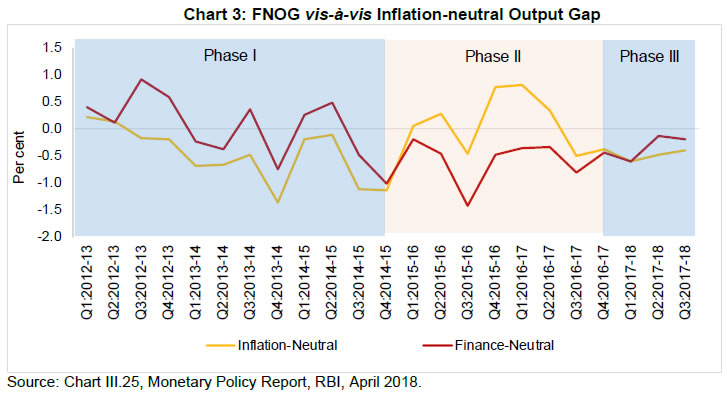
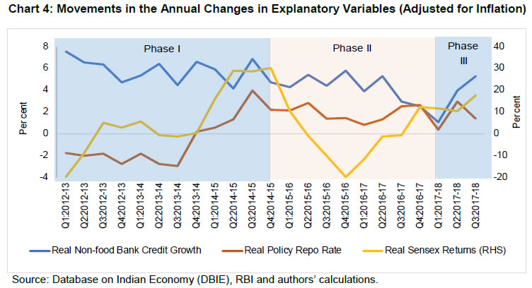
A further detailed comparison of the FNOG vis-à-vis the inflation-neutral output gap for India shows that there are crucial differences between the two as evident in three phases (Charts 3 and 4).
-
In phase I (Q1:2012-13 to Q4:2014-15), the FNOG was above the inflation-neutral output gap and mostly positive as this period witnessed episodes of high credit growth and real stock market returns. However, the inflation-neutral output gap was negative throughout.
-
In Phase II (Q1:2015-16 to Q4:2016-17), the FNOG remained in the negative territory and much below the inflation-neutral output gap, mainly on account of subdued financial conditions in the form of low credit growth due to stressed balance sheets of banks and corporates as well as depressed stock market as reflected in negative real stock market returns.
-
In Phase III (2017-18), the FNOG remained negative but tended to close, reflecting revival of credit growth and buoyant stock market conditions. During this phase, the inflation-neutral output gap also remained negative and tended to close, but at a slower pace than the FNOG.
 The role of financial variables in explaining the FNOG is also evident from the historical variable decomposition of the FNOG, portraying the contribution of various factors on its evolution (Chart 5). For instance, credit growth and stock market returns contributed negatively to the evolution of the FNOG in Phase II (Q1:2015-16 to Q4:2016-17). However, in Phase III (2017-18), financial market variables contributed positively to the FNOG.
IV. Conclusion
The estimation of output gap incorporating financial market information has gained popularity in recent years. The FNOG measure, which incorporates financial market indicators, provides a useful addition to a set of indicators used for assessing the state of economy for policy purposes. The inflation-neutral output gap measure has relied on inflation as the source of imbalances in the economy. However, this measure failed to capture the imbalances arising from high credit growth and asset market returns in the pre-GFC period. The FNOG takes into account financial sector indicators, such as credit and asset market variables, for estimating the output gap.
The FNOG estimated for the period Q1:2006-07 to Q3:2017-18 in the Indian context provides useful insights into the state of the economy, especially in periods of high/low credit growth and stock market returns, which conventional measures do not. The FNOG remained negative from Q3:2014:15 onwards, but almost closed by Q2:2017:18. A comparison of the FNOG with the inflation-neutral output gap suggests that during Q1:2012-13 to Q4:2014-15, the FNOG remained above the inflation-neutral output gap. However, from Q1:2015-16 to Q4:2016-17, the FNOG remained much below the inflation-neutral output gap, driven mostly by low credit growth. From Q1:2017-18, both the inflation-neutral output gap and the FNOG remained negative but tended to close gradually. However, the FNOG tended to close faster than the inflation-neutral output gap.
Estimates of both potential output and output gap are unobservable variables, and their estimates can be sensitive to the selected approach. The RBI staff, therefore, undertakes an assessment of the output gap using alternative estimation approaches, supplemented by information from various surveys and other macroeconomic variables, to draw more robust inferences on the stage of the business cycle.
References
C. Borio, P. Disyatat and M. Juselius, “Rethinking Potential Output: Embedding Information about the Financial Cycle,” BIS Working Papers, 404, (February 2013).
A. Okun, “Potential GNP: Its Measurement and Significance,” In Proceedings of the Business and Economic Statistics Section, Washington: American Statistical Association, (1962), pp. 98-104.
D. P. Rath, P. Mitra, and J. John, “A Measure of Finance-Neutral Output Gap for India”, RBI Working Paper Series, WPS (DEPR), March (2017).
Annex
Inflation-Neutral Output Gap and Finance-Neutral Output Gap - Measurement
This technical annex details the analytical setup of univariate statistical filter, inflation-neutral and finance-neutral measures of output gap.
The Hodrick-Prescott (HP) Filter is one of the most popularly used univariate statistical filter to estimate the output gap. This filter is based on weighted moving average of the observations putting greater weights for the observations close to the beginning and end of the sample period. This method obtains potential output (Ȳt) by minimising the following function,
 The first term is the sum of squared deviations of Yt from the trend, i.e, potential output (Ȳt), which penalises the cyclical component. The second term is a multiple λ of the sum of squares of the second difference of potential output (Ȳt). The second term penalises variations in the growth rate of potential output (Ȳt). The larger the value of the positive parameter λ, the greater the penalty and the smoother will be the resulting potential estimate. Hence, in the limiting case if λ = 0 when there is no penalty for smoothing, the filter produces the trend as the series itself. On the other hand, if λ is very high, then there will be a high weightage for smoothing and the trend will be a straight line.
I. Inflation-Neutral Output Gap
The output gap (yt) is defined as the deviation of real output4 in log terms (Yt), from its potential level (Ȳt).
In addition to the equations (2) and (3), output gap has been modeled as an auto regressive process as follows:
In the inflation-neutral approach, the sustainable level of output has been defined as the level of output compatible with low and stable inflation (Okun, 1962). Therefore, to estimate an inflation-neutral output gap measure, Phillips Curve equation for inflation is added, which links the evolution of the output gap to observable data on inflation (πt) according to the following process.
The estimated output gap from this framework (using equations 2 to 5) is consistent with the inflation level and known as inflation-neutral output gap.
II. Finance-Neutral Output Gap
In this framework, financial variables (real bank credit growth and real stock market return) along with real interest rate are used as explanatory variables for the output gap. The modified output gap equation after incorporating these variables is given below:
where Xt = (rt, bct, sensext) ; rt : real policy rate; bct : real bank credit growth; sensext : real stock market return proxied by BSE Sensex. The estimated output gap from this framework (using equations 2, 3 and 6) is known as finance-neutral output gap since this measure controls for the movement in the financial variables.
The system of equations is estimated using Quasi Maximum Likelihood (QML) method in a state space framework by applying Multivariate Kalman Filter. Kalman filtering, named after Rudolf E. Kálmán, is an algorithm that uses a series of measurement variable(s) observed over time, containing statistical noise and other inaccuracies, and produces estimates of unobserved variable(s).
|