|
Abstract - Given the key role played by sovereign bond yields in the transmission of monetary policy, this study empirically examines the drivers of government bond yields in India. Policy rate is found to be a key driver of bond yields of short-term securities, and the impact on yields weakens as the tenure of the bonds increases. Estimates in this study suggest that an increase of 100 basis points (bps) in the policy rate could, over time, lead to an increase of around 95 bps in yields of 15-91 days residual maturity Treasury Bills and around 20 bps for 10-year government securities. The size of the government’s borrowing programme, foreign portfolio investments in the domestic bond market and foreign bond yields are also found to move domestic government bond yields, although the impact of these factors differs across maturities.
I. Introduction
Between December 2014 and August 2017, the Reserve Bank cut its policy rate by 200 basis points (bps) and the yield on 10-year Central government securities (G-Secs) fell by around 140 bps. Conversely, between August 2017 and May 2018, the yield on 10-year G-Secs increased by around 140 bps, even as the Reserve Bank’s policy repo rate was unchanged at 6 per cent over this period. Yields on short-term treasury bills (TBs) over both these episodes, however, moved broadly in tandem with the policy repo rate (Chart 1). Similar dynamics are observed in advanced economies such as the United States (US) (Chart 2).
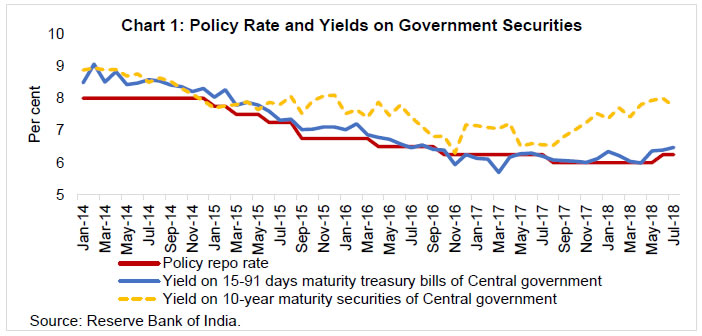
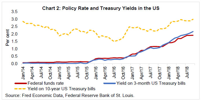 The weak correlation between the policy rate and the yields on longer-dated government bonds has been observed in the past and dubbed as “conundrum” (Greenspan, 2005). According to Fama (2013), changes in the federal funds rate target have little effect on the US long-term government bond yields, and there is substantial uncertainty in their impact on short-term treasury bills yields; rather, the Federal Reserve (Fed) responds to changes in market rates.
The government securities market, given its risk-free nature, is a key conduit for transmission of monetary policy impulses to the broader real economy by the virtue of it being a benchmark for pricing of other financial instruments, such as, commercial paper, corporate bonds, and derivative products. Against this backdrop, this study attempts to empirically assess the role of various factors that impinge upon the yields of G-Secs across the maturity spectrum in the Indian context.
II. Yield Movements: Potential Drivers
Changes in the central bank’s policy rate impact a host of interest rates across the spectrum, including yields on short-term treasury bills, and medium- to long-term bonds. Apart from the central bank’s policy rate, a number of factors can impact bond yields with a likely differential impact on bonds of different maturities. First, the central bank’s policies on liquidity provision to the banking system can add to the channel operating through the policy rate (Dua, Raje and Sahoo, 2003; Singh, 2011). Open market operations, foreign exchange market operations by the central bank, public’s demand for currency, and changes in cash reserve ratio (CRR) impact liquidity available with banks for investment in alternative avenues (including in government bonds), and this can impact bond yields. These factors would get reflected in repo/reverse repo operations under the Reserve Banks’ Liquidity Adjustment Facility (LAF) window. Thus, not only the central bank’s policy interest rate, but its liquidity stance can also be an important determinant of bond yields.
Second, if the government’s deficit increases, it might need more borrowings from the market to finance the deficit. More borrowings would increase the supply of bonds in the market, thereby reducing the prices of these bonds and increasing the yields (as bond prices and yields are inversely related). The regulatory requirements, such as, statutory liquidity ratio (SLR) also influence the investment demand for G-Secs and their yields. Moreover, a sizable proportion (more than 50 per cent) of the banks’ SLR holdings is under the 'Held to Maturity', and it provides cushion to banks from valuation changes (Acharya, 2018). A large share of holdings under the HTM category can impact market liquidity and yields. Yields can also move in response to shifts in the investors’ relative preference for short- and long-maturity bonds. For example, portfolio adjustment by long-term investors (in insurance and pension sectors) aimed at containing duration mismatches – rather than monetary easing by the European Central Bank - was a key factor for the sharp decline in long-term sovereign bond yields in Europe in 2014 (Shin, 2017).
Third, investments by non-residents in the domestic bond market increase demand for the bonds, and hence can reduce the yields, and vice versa when investors sell their holdings. In India, foreign portfolio investors (FPIs) have been permitted to invest in domestic debt markets, and these investments are, among others, subject to prudential limits and minimum maturity requirements, which have varied over time. Global financial market uncertainty and the associated risk-on risk-off tendency among foreign investors can lead to sudden and large shifts in investments and domestic yields.
Fourth, as Charts 1 and 2 show, there is some evidence of co-movement of long-term yields in India with those in the US. These dynamics seem to be an illustration of the global financial cycle hypothesis - i.e., the financing conditions and the monetary policy stance in the major global financing centres (such as the US) set the tone for the rest of the world, regardless of the exchange‐rate regime - posited by Rey (2015). In an environment characterised by enhanced financial integration across countries, the global financial cycle in capital flows, asset prices and in credit growth is driven by monetary policy in the centre country (the US), which affects the leverage of global banks, capital flows and credit growth in the international financial system. Therefore, the sovereign bond yields in the US and other major advanced economies can have a direct impact on domestic bond yields in India.
Thus, apart from the central bank’s policy rate, the potential drivers of government bond yields include liquidity conditions in the domestic banking system, government’s deficits and borrowing requirements, non-resident investment flows into domestic bonds, and sovereign bond yields in the US. Since the relationship of short- and long-term yields with the policy rate is quite divergent (as seen in Charts 1 and 2), this study explores the dynamics of the yield curve across a range of maturities (10-year, 5-year and 1-year residual maturity securities and 15-91 days residual maturity treasury bills) for a better understanding of the yield dynamics.
In principle, monetary policy changes are expected to have more impact on short-term yields vis-à-vis long-term yields. To elaborate, according to the expectations hypothesis of the term structure, the long-term interest rates are the average of current and expected future short-term interest rates plus some risk/term premia (for the uncertainty associated with future short-term rates) (Bernanke, 2015).2 If the economy is growing above its potential and there are inflationary pressures, then the central bank is expected to start tightening today. Short-term rates increase proportionally and quickly. Over time, markets expect future growth slowdown, easing of inflationary pressures, and a reversal of the central bank tightening stance. The medium and long-term rates (being expectations of future short-term rates), thus, can be expected to move less than the change in short-term rates. Hence, monetary policy actions can have a stronger and quicker impact on near-term rates, with the magnitude of the impact waning as the maturity increases (Estrella and Trubin, 2006). However, a variety of factors, such as, time-varying term premium (in turn, due to changing expectations of future growth and/or inflation), deepening of the financial sector, and changes in the relative preference of investors for shorter maturities vis-à-vis longer maturities can lead to deviations from the expectations hypothesis.
III. Yield Movements: Empirical Analysis
Based on the discussion in the previous section and data availability, we postulate that the yields on G-Secs are likely driven by: (i) policy rate (EFF); (ii) cash reserve ratio (CRR); (iii) banks’ recourse to the liquidity adjustment facility (LAF_Y) [positive (negative) sign for LAF_Y indicates surplus (deficit) liquidity conditions, that is, the Reserve Bank is in a liquidity absorption (injection) mode]; (iv) government’s gross market borrowings (GMB_Y); (v) foreign portfolio investment (net inflows) in domestic debt securities (FPID_Y)3; and, (vi) yields on one-year maturity treasury bonds in the US (GUS). Over the earlier part of the sample period, the domestic prices of petrol and diesel were administered and the change in domestic prices of these products in response to changes in international crude oil prices was partial and lagged, with implications for government’s deficit and borrowings and bond yields. The quarterly variation (annualised) in crude oil prices in rupee terms (ΔOil) is, therefore, also included as an explanatory variable in the empirical analysis. The sample period of the empirical exercise is April 2004-March 2018.
Summary Statistics
Summary statistics of the key variables are provided in Table 1. Over the sample period, the yields on 15-91 days TBs (G15-91), 1-year G-secs (G1Y), 5-year G-secs (G5Y), and 10-year G-secs (G10Y) averaged 6.7 per cent, 7.0 per cent, 7.5 per cent and 7.7 per cent, respectively - the higher the maturity period, the higher is the yield. This upward sloping yield curve seems consistent with the earlier noted expectations hypothesis. The short-maturity yields exhibit more volatility vis-à-vis long-term yields, in accordance with the trends observed in Charts 1 and 2.
| Table 1: Summary Statistics |
| (Per cent) |
| Variable |
Mean |
Standard Deviation |
Minimum |
Maximum |
| Policy Rate |
6.4 |
1.5 |
3.3 |
9.0 |
| 15-91day T-bill rate |
6.7 |
1.6 |
3.1 |
11.1 |
| 1yr G-sec Yield |
7.0 |
1.3 |
4.0 |
10.0 |
| 5yr G-sec Yield |
7.5 |
0.9 |
4.9 |
9.5 |
| 10yr G-sec Yield |
7.7 |
0.8 |
5.1 |
9.4 |
Note: Sample period is April 2004 to March 2018.
Source: Authors’ estimates. |
Modelling Approach
In contrast to the regression framework (which estimates one maturity at a time), the VAR framework models all the four maturities (G15-91D, G1Y, G5Y, G10Y) as a system, recognising that there might be some common factor amongst the yields being studied. As noted earlier, Fama (2013) presents some evidence that the target federal funds rate changes in response to market rates, or in other words, markets anticipate future changes in the fed funds rate and the Fed just accommodates these market dynamics. The VAR framework can address this concern, since its focus is on studying the dynamics of yields in response to an unanticipated change in the policy rate. Conversely, the regression framework focuses on the dynamics of yields in response to a systematic (expected) conduct of monetary policy. Thus, the VAR analysis supplements the regression analysis and can help us to draw more robust inferences.
While the regression analysis employs quarterly variables, the VAR analysis is based on monthly data to study the dynamics more closely. The sample period for the analysis is April 2004-March 2018 in both the estimation approaches. Unit root tests suggest some ambiguity on the stationarity property of the four yields being studied.6 For robustness purposes, the regression analysis uses such variables in a first-difference form (i.e., quarter over quarter changes), while the VAR analysis is based on data in levels. 7
Estimation Results
Regression results indicate that monetary policy has a relatively stronger effect on short-term yields vis-à-vis long-term yields. An increase of 100 bps in the policy rate, ceteris paribus, increases the yield on 15-91 days maturity TBs by around 85 bps, and the impact reduces as the maturity increases (around 50 bps on 1-year securities, around 25 bps for 5-year securities and less than 10 bps on 10-year securities) (Table 2).8 Other variables also have the expected impact on yields, although the magnitude differs across the various maturities. First, the monetary/liquidity variables (cash reserve ratio and liquidity adjustment facility) have the expected impact. Second, higher gross market borrowings by the government push up yields by about 3 bps for every one percentage point increase in the borrowings/GDP ratio. Third, over the sample period, higher crude oil prices are found to put upward pressure on yields. Fourth, an increase of one percentage point in foreign portfolio investment in debt instruments (per cent to GDP) softens one, five and 10-year domestic bond yields by 10-23 bps, with no significant impact on short-term TBs. Unlike the policy rate, foreign portfolio investments impact longer-term yields more vis-à-vis shorter-term yields. These results seem consistent with the policy framework on FPI flows, which has over the sample period tended to encourage such investments into longer-term yields through the stipulation of minimum maturity requirements. Finally, an increase of 100 bps in the 1-year US Treasury bonds pushes up domestic G-Sec yields by around 25-30 bps, with a somewhat higher impact on longer-maturity bonds, providing some evidence to the global financial cycle, as alluded to earlier.
| Table 2: Determinants of Yields on Government Securities |
| Explanatory Variables |
Dependent Variable |
| ΔG15_91 |
ΔG1Y |
ΔG5Y |
ΔG10Y |
| Constant |
0.00 |
-0.14 |
0.07 * |
-0.08 |
| |
(0.08) |
(-1.47) |
(1.91) |
(-1.16) |
| ΔEFFt |
0.84 *** |
0.47 *** |
0.23 *** |
0.07 * |
| |
(13.81) |
(5.94) |
(3.40) |
(1.90) |
| ΔLAF_Yt |
-0.18 ** |
-0.17 *** |
-0.20 *** |
-0.23 *** |
| |
(-2.46) |
(-4.04) |
(-3.33) |
(-3.81) |
| ΔCRRt |
|
0.29 *** |
0.21 *** |
0.25 *** |
| |
|
(4.09) |
(3.44) |
(4.46) |
| GMB_Yt |
|
|
|
0.03 ** |
| |
|
|
|
(2.35) |
| GMB_Yt-1 |
|
0.03 ** |
|
|
| |
|
(1.99) |
|
|
| ΔOILt |
|
0.002 *** |
0.003 *** |
0.003 *** |
| |
|
(3.24) |
(4.40) |
(4.72) |
| FPID_Yt-1 |
|
-0.10 ** |
-0.16 *** |
-0.23 *** |
| |
|
(-2.05) |
(-3.57) |
(-5.70) |
| ΔGUSt |
|
0.23 *** |
0.23 *** |
0.32 *** |
| |
|
(3.85) |
(3.59) |
(4.37) |
| ΔG1Yt-2 |
|
0.11 ** |
|
|
| |
|
(2.04) |
|
|
| ΔG5Yt-1 |
|
|
-0.25 *** |
|
| |
|
|
(-3.39) |
|
| ΔG10Yt-1 |
|
|
|
-0.24 *** |
| |
|
|
|
(-3.90) |
| |
|
|
|
|
| R-bar2 |
0.78 |
0.87 |
0.76 |
0.78 |
| LB-Q (p-value) |
0.54 |
0.28 |
0.22 |
0.64 |
| |
|
|
|
|
Notes:
***, ** and *: Significant at <1%, <5% and <10% levels, respectively.
Figures in parenthesis are t-statistics based on heteroscedasticity and autocorrelation consistent (HAC)-corrected standard errors. LB-Q is p-value of Box-Pierce-Ljung Q-statistic for the null hypothesis of no residual autocorrelation up to 4 lags.
Variables are defined as follows:
G15-91 = Yields on central government treasury bills of residual maturity of 15-91 days;
G1Y, G5Y and G10Y = Yields on central government securities of residual maturity of 1-, 5- and 10-years, respectively; CRR = Cash reserve ratio; EFF = Policy rate; LAF_Y = Outstanding LAF balance (% of GDP); GMB_Y = Central government market borrowings (% of GDP); OIL = International crude oil price (rupee terms); FPID_Y = Net foreign portfolio investments in debt (% of GDP); YUSG = Yield on one-year G-sec of the US.
Sample period for the estimation is April-June 2004 to January-March 2018.
Source: Authors’ estimates. |
Vector Autoregression Results
The vector autoregression (VAR) analysis employs the same variables as the regression analysis in the previous sub-section and the results are qualitatively similar, i.e., the impact of policy rate changes on G-secs is more on shorter-dated securities and less on longer-dated securities (Chart 3).9 In quantitative terms, the initial impact on 15-91 days maturity TBs in the VAR analysis is similar to the results from the regression approach, while the effect on one-, five- and 10-year securities is somewhat higher.10
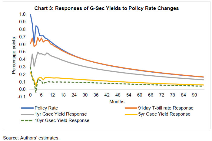 Following a shock to the policy rate, the impact on shorter maturities (15-91 days and one year) builds over time and the peak effect occurs with a lag of around six months. For five- and 10-year maturities, the dynamics suggest some over-shooting of yields in the initial month, as markets seem to absorb the news and implications of a rate hike; the over adjustment of yields is corrected in the next couple of months and there is a smooth adjustment in the subsequent months. The cumulative pass-through11 of a shock increase of 100 bps in the policy rate after 12 months is 86 per cent, 60 per cent, 20 per cent, and 15 per cent for 15-91 days, one-year, five-year and 10-year maturity securities, respectively.12 Over time, the pass-through is almost full (96 per cent) for 15-91 days maturity securities, and increases to 72 per cent, 30 per cent and 21 per cent for one-, five- and 10-year maturity securities, respectively. These are average responses over the sample period and the actual response at any time, as Chart 1 suggests, would depend upon a variety of other domestic and global factors. Overall, the empirical evidence using alternative estimation techniques in this study indicates that, while the policy rate is an important driver of short-term yields, the medium- and long-term yields respond more to a variety of non-monetary factors.
IV. Concluding Observations
Sovereign bond yields are an important conduit for effective transmission of monetary policy to the spectrum of financial prices and the broader real economy. This study empirically examines the drivers of domestic government bond yields employing alternative estimation techniques. Policy rate is found to be a key driver of yields of short-term government securities, but its impact on yields weakens as the maturity of bonds increases. While the long-run pass-through from policy rate changes is almost complete in the case of shorter maturity securities, the pass-through is 20-30 per cent for longer-term bonds. The size of the Central government’s borrowing programme, foreign portfolio investments in the domestic bond market and foreign bond yields are also found to move domestic bond yields, though the impact of these factors differs across maturities.
References
Acharya, Viral V. (2018), “Understanding and Managing Interest Rate Risk at Banks”, Reserve Bank of India Bulletin, February, pp.7-17.
Bernanke, Ben (2015), “Why are Interest Rates so Low, Part 4: Term Premiums”, available at https://www.brookings.edu/blog/ben-bernanke/2015/04/13/why-are-interest-rates-so-low-part-4-term-premiums/
Dua, Pammi, Nishita Raje and Satyananda Sahoo (2003), “Interest Rate Modelling and Forecasting in India”, Development Research Group Study 24, Reserve Bank of India.
Estrella, Arturo and Mary Trubin (2006), “The Yield Curve as a Leading Indicator: Some Practical Issues”, Current Issues in Economics and Finance, Vol. 12(5), Federal Reserve Bank of New York.
Fama, Eugene (2013), “Does the Fed Control Interest Rates?”, The Review of Asset Pricing Studies, Vol. 3(2), pp.180-199.
Greenspan, Alan (2005), “Testimony of Chairman Alan Greenspan: Federal Reserve Board’s Semiannual Monetary Policy Report to the Congress.” Board of Governors of the Federal Reserve.
Rey, Hélène (2015), “Dilemma not Trilemma: The Global Financial Cycle and Monetary Policy Independence”, NBER Working Paper No. 21162.
Shin, Hyun (2017), “How Much Should We Read into Shifts in Long-dated Yields?”, Speech at US Monetary Policy Forum, available at https://www.bis.org/speeches/sp170303.htm
Singh, Bhupal (2011), “How Asymmetric is the Monetary Policy Transmission to Financial Markets in India?”, Reserve Bank of India Occasional Papers, Vol. 32(2), pp.1-37.
|