Press Release RBI Working Paper Series No. 03
Global Spillovers and Monetary Policy Transmission in India
@Michael Debabrata Patra,
Sitikantha Pattanaik,
Joice John and
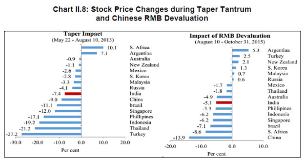
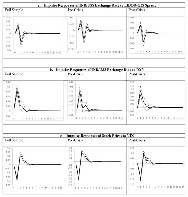
Harendra Kumar Behera Abstract Do global spillovers clog transmission channels of monetary policy through domestic financial markets? Drawing on stylised facts and using a dynamic factor model to develop an indicator of global spillovers (IGS), a time-varying parameter vector autoregression (TVP-VAR) model results indicate that monetary policy transmission through the money market is complete even in the face of global spillovers. In the debt market, global spillovers affect transmission and can even produce overshooting and over-corrections, but domestic factors such as market microstructure have a stronger influence. In the credit market, spillovers have no statistically significant influence on transmission to lending rates. Asset quality of banks and financial deepening play a more important role. JEL Classification: C54; E52; E58 Key Words: Global Spillovers, Monetary Policy Transmission, Dynamic Factor Model, M-GARCH, Time-Varying Parameter VAR With the world’s largest economies setting divergent courses for monetary policy, will spillovers from this transatlantic schism imprison interest rates in emerging market economies (EMEs) like India that are reasonably well integrated into the global financial cycle? Will it be possible for these countries to conduct independent monetary policy as capital and asset prices are stirred up by the core financial centres? These questions form the theme of this paper. We ask them in the context of a rapidly proliferating strand in the empirical literature that is finding increasing evidence of significant spillovers effects not just for fixed income markets and longer-term interest rates (Obstfeld, 2015; Sobrun and Turner, 2015; Turner, 2014; Miyajima et al., 2014) but for short-term interest rates and policy rates as well (Hofman and Takats, 2015; Edwards, 2015; Takats and Vela, 2014; Gray, 2013). Furthermore, as this evidence accumulates, the channels of propagation are becoming clearer and as a consequence, more real and present for open EMEs – global economic and financial integration (Hofman and Takats,2015); investor arbitrage playing out through both EME allocations in globally mobile funds and foreign participation in local markets (Barroso, Kohlscheen and Lima, 2014); foreign currency denominated credit (He and McCauley, 2013); and increased sensitivity of EME policy makers to volatility in capital flows and exchange rates. While considerable heterogeneity is found in these effects across EMEs (Chen et al., 2015), the constraining effects of spillovers on domestic monetary policy is observed irrespective of the exchange rate regime (Rey, 2015). The persuasiveness of this strand notwithstanding, there is a contrarian view too – why wouldn’t there be one? In the long run we are all economists2 - that seems to be standing up to the tests of the episodes of volatility in 2015 relative to the ‘taper caper’3. It is argued that the concept of monetary policy independence needs to distinguish between the ability to set monetary policy independently and the willingness to do so, the latter implying the extent to which external developments enter policy reaction functions of EME central banks and the coefficients attached to them. The effects of spillovers or contagion when appropriately measured seem to be less severe for EMEs than generally assumed or observed in financial phenomena such as co-movements in interest rates across borders (Disyatat and Rungcharoenkitkul, 2015). First, in the taper caper and its aftermath, several EMEs allowed exchange rate adjustments, some even large and apparently disruptive, but this enabled them to set domestic interest rates to domestic conditions. The exchange rate change was a measure of the importance of external developments in their reaction functions and their willingness to accommodate them rather than a loss of monetary policy independence. By the same logic, several EMEs are regarded as engaged in pursuing exchange rates that reflect domestic goals – competitive depreciations. Both interest rates and exchange rates can be regarded as instruments that serve domestic objectives. Secondly, some EMEs with large reserves actively intervened to stem turmoil in their foreign exchange markets and by all counts succeeded, effectively preventing the trilemma from breaking down to a dilemma a la (Rey, 2015) and setting in motion what has been termed as quantitative tightening (QT) that supported domestic conditions. Also, many EMEs continue to retain both macro-prudential and administrative policies that can influence capital flows in both directions, and this instrument is acknowledged to secure monetary policy autonomy. Thirdly, several EMEs including India have repaired and strengthened macroeconomic fundamentals and policies. As events of 2015 relative to the taper caper showed, these actions buffered their economies considerably, contrary to the view that in the face of spillovers, fundamentals do not matter (Eichengreen and Gupta, 2013)4. This view itself has been questioned by evidence of investors differentiating among EMEs based on fundamentals, and especially in favour of deeper markets and tighter macro-prudential policies (Mishra et al., 2014a). Moreover, differentiation was found to have set in early and persisted for some time (Ahmed et al., 2014). In fact, this has led several central banks to urge the US Fed to stop stoking speculation and to ‘just get on with it’ in normalising US monetary policy (Weidman, 2015; Singh, 2015; Shanmugaratnam, 2015; Rajan, 2015). This paper is an empirical exploration of these two sets of issues in the Indian context. The rest of the paper is organised into five sections. The next section presents stylised evidences on channels of contagion and their impact on financial markets in India which transmit monetary policy. Section III develops a measure of global spillover. Section IV presents and discusses empirical results. Section V concludes the paper with implications for conducting monetary policy in an open EME. Section II: Living with Spillovers: The Indian Experience A stable and efficient financial market continuum is a sine qua non for monetary policy transmission: policy signals conveyed through interest rate changes or monetary conditions more generally are transmitted outward through financial market variables until they reach longer-term rates and eventually aggregate demand. In a spillover rich environment, however, the behaviour of the spectrum of domestic interest rates and asset prices is altered, sometimes significantly and persistently. Perturbations in India’s domestic financial market segments during the period of study which coincides with UMPs as well as high intensity global shocks such as the European sovereign debt crisis, the taper caper, the bund tantrum and the Chinese devaluation is the focus of this section. The discussion is arranged in terms of the stages in which each market segment transmits monetary policy impulses. Money Market In India, the money market provides the first leg of monetary policy transmission – policy rate changes impact the uncollateralised weighted average call money market rate (WACR) instantaneously and, in turn, all other money market rates evolve around the WACR with varying spreads (Chart II.1a). Typically, the money market is insulated from external shocks, essentially due to active liquidity management by the RBI (Chart II.1b), and is driven by domestic factors such as transactions in government balances, currency demand and the like. The absence of long-lived disruptions in interbank overnight and money markets is largely corroborated in the country experience (Moreno and Villar, 2010). 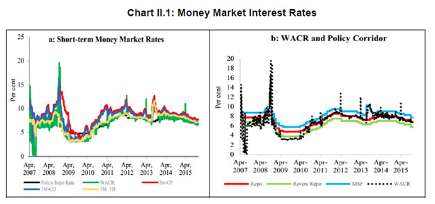 In India, the spread between the WACR and the policy rate tends to widen around the end of the financial year when banks’ balance sheet adjustments increase the demand for storing liquidity. During the global financial crisis and the taper caper, however, money market spreads widened significantly, dispelling the sense of insulation and provoking unconventional policy responses (Chart II.2). In response to the former, the RBI lowered its policy repo rate by 425 bps cumulatively and injected liquidity/opened up liquidity windows aggregating to 10 per cent of GDP to avert a liquidity freeze. In May-September 2013 as the taper caper hit EMEs, the RBI again responded, perhaps the only country to react unconventionally other than Turkey. It widened the policy corridor by raising the standing facility rate by 200 bps and drained out liquidity by tightening reserve requirement maintenance and restricting access to liquidity under normal repos. These actions effectively raised the WACR by 300 bps, with a view to preventing free fall of the rupee (Pattanaik and Kavediya, 2015). Significantly, the policy rate was kept unchanged to reflect the domestic focus of monetary policy through these troubled times. On both occasions, exceptional monetary measures were normalised quickly. 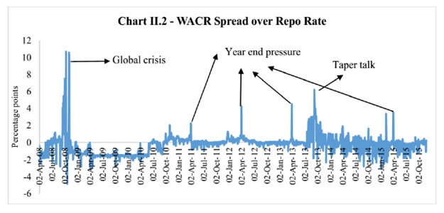 Money markets in India are also shielded from global spillovers by statutory liquidity ratio (SLR) requirements which entail that banks maintain a fixed proportion of liabilities in gilts – currently 21 per cent. SLR maintenance in excess of the statutory requirement allows banks to get access to central bank liquidity as well as to secured markets, thus obviating a collateral constraint. Furthermore, banks largely fund themselves through retail deposits rather than wholesale funding, which has been identified elsewhere as a source of vulnerability to external contagion (Mesquita and Toros, 2010). Three-month T-Bill yields, like other short-term interest rates, have closely tracked the policy repo rate but for the two major global events mentioned earlier. In this context, however, a caveat is in order – during the global financial crisis, the reverse repo rate or the floor of the policy corridor became the effective policy rate whereas after the taper talk episode, the MSF rate or the ceiling was the effective policy rate and both were orchestrated by monetary policy. Therefore, even during these two event shocks, it is the domestic monetary policy stance that influenced short-term rates. Bond Market Much of the international debate in the empirical literature highlights co-movement of long-term yields as an example of possible loss of independence of domestic monetary policy. India’s 10 year G-sec yields, in fact, show high degree of co-movement with US and German government bond yields, but only during three episodes – the global financial crisis (GFC), the taper caper and the bund tantrum (Chart II.3a). During the first two of these episodes, however, G-sec bond yields largely reflected the domestic monetary policy stance, which adjusted to insulate domestic macroeconomic conditions, and quite successfully so (Chart II.3b).  The Indian experience with regard to spillovers and g-sec yields is also borne out in the literature in which a broad consensus suggests that when markets are on edge, they pay greater attention to country-specific fiscal fundamentals, rather than global correlations (Jaramillo and Weber, 2013a). In the short-run, however, financial vulnerabilities may matter in spread formation (Bellas et al., 2010), but here too, it is important to recognise country-specifics5. First, the large non-resident holdings of locally issued domestic government bonds, which exposed domestic bond markets to rising co-movements and spillovers in other countries – flights to safety and reaching for yield (Soburn and Turner, 2015) are not found in India: the share of foreign portfolio investors in the stock of government bonds is less than 5 per cent6. Secondly, the recent surge in direct issuances of US dollar denominated bonds by EME corporates in international capital markets – which more than doubled since 2008 – has largely bypassed India, which accounted for only 5 per cent of this surge7 (Chart II.4a). Much of these issuances were driven by the lure of carry trade, i.e., financial risk taking rather than for real investment (Bruno and Shin, 2015). Thirdly, unlike in some EMEs – Poland; Mexico; Hungary (Moreno, 2010) - changes in short-term interest rates appear to be the lead driver of changes in nominal G-sec yields in India (Akram and Das, 2015). This is also found in broader surveys of country experiences, although stable inflation expectations tend to dampen the direct impact (Mohanty and Turner, 2008).  Corporate bond yields in India essentially track the 10-year G-sec yield, with changing risk spreads over time (Chart II.4b). But for occasional deviations of risk spreads from normal levels, the evolution of bond yields is consistent with domestic monetary policy cycles. Corporate bond yields tend to follow g-sec yields in overshoots in response to global shocks; the speed of adjustment is also faster. Credit Market The recent literature also documents the credit channel of spillovers across EMEs in emerging Europe (Brzoza-Brzezina, et al., 2010) and Asia (He and McCaulay, 2013): low interest rates on major currencies provide an incentive to substitute foreign currency credit, mostly dollar-denominated, for local currency credit. In addition, expectations of currency appreciation provide a further incentive for external borrowing. To the extent that foreign currency credit in the region is priced off global benchmarks, monetary accommodation in the key currencies makes for immediately easier financial conditions wherever there is a substantial stock of foreign currency credit (Borio et al., 2011). In the Indian context, however, this channel has so far been muted. India’s financial system is still bank-dominated8, and therefore, bank lending rates still remain important in monetary policy pass-through, notwithstanding a proliferation of nonbanking sources of finance for corporates, including from international markets. A number of factors impinge upon this transmission, as in other countries, and have a bearing on the incentive structures that banks face in determining the speed and completeness of the pass-through. The overall quality of the regulatory environment, extent of dollarisation, depth of financial development, asset quality, competition in the banking space, exchange rate flexibility and the inflation environment have been identified as factors affecting policy transmission to bank lending rates in the country experience (Mishra et al., 2014b). In India, administered interest rates, rigidities in repricing of deposits, interest rate subventions, the coexistence of large informal finance, fiscal dominance, including through statutory pre-emptions and asset quality concerns are additional dimensions that delay and dilute the pass-through. In spite of these impediments, the policy repo rate continues to condition the evolution of nominal weighted average lending rates by influencing the cost of funds – wholesale and retail. Global spillovers proxied by VIX have a muted impact, if at all (Chart II.5). 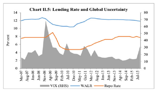 Another important characteristic that limits external spillovers to credit markets in India is the miniscule share of non-resident participation in deposits and loans. Non-resident deposits (excluding rupee deposits), which are priced off a foreign interest rate, constitute barely 3 per cent of banks’ total liabilities. On the assets side, 3 per cent of outstanding bank assets are externally sourced. Banks’ access to external finance is governed by prudential regulations that limit it to 100 per cent of their tier 1 capital. Moreover, open positions and gap limits attract capital charges. In contrast to the surges and retrenchments of foreign funded bank credit in several emerging economies in Europe (Guo and Stepanyan, 2011), the major driver of credit in India, both before and after the global crisis, has been domestic deposits which largely determine the cost of funds and thereby the base rate. Wholesale funding plays a role only at the margin as does the risk premium both of which could be subjected to spillovers and global uncertainty. FX Market and Equity Prices The exchange rate channel is widely regarded as the most potent channel of transmission of spillovers to the domestic economy (Aizenman and Binici, 2015). In the context of UMPs, the impact on exchange rates of EMEs can occur through several channels some of which are intertwined. Externalities can flow through the quantity channel - as AE central banks engage in quantitative easing, their currencies depreciate. Ample liquidity and low returns push out flows to EMEs in a search for yields, causing appreciation in the latter’s exchange rates unrelated to fundamentals (Cerutti, et al., 2015). Spillovers can take a more direct route – changes in bond yield differentials and equity valuations may provoke investor repositionings and asset re-allocations with immediate effects on exchange rates. Finally, there is the expectations channel, as vividly demonstrated at the time of the taper caper. UMPs announcements can be ‘lumpy’ news for markets; in the case of incoming data dependent UMPs, even expectations of announcements can trigger surprises and sizable exchange rate adjustments (Chua et al., 2013). While there has been considerable focus on the expectations channel of transmission of spillovers to the exchange rate, balance sheet effects have become important in the context of elevated levels of foreign currency borrowings and leverage by corporates (Bacchetta and and Merrouche, 2015). In India, movements in the exchange rate have largely evolved in line with domestic priors, attributable to the relatively lower reliance closed nature of the economy on the external finance and the exchange rate policy of the RBI which intervenes in the forex market to smooth volatility. In the post-crisis years, however, the growing importance of portfolio investment flows has tended to impact episodes of volatility in both the foreign exchange market and the equity market (where portfolio equity flows account for about 20 per cent of market capitalisation, 40 per cent of turnover and 45 per cent of the floating market capitalisation), which are amplified by risk-on risk-off shifts. Not surprisingly, the forex market and the stock market have co-moved to a degree not observed in pre-crisis years. Spillovers embedded in portfolio flows into equity and bond markets have triggered large exchange rate and stock market adjustments only when fundamentals were misaligned as at the time of the global financial crisis and again at the time of the taper caper. Even after the large nominal depreciation that followed taper talk and took India into the fragile five, the extent of real appreciation remained significant, reflecting persistently high inflation. In other occasions, left tail events have provoked step adjustments but of diminishing and more gradual magnitudes, at least in relation to the EME peer experience. In 2015, India was least impacted among major emerging economies by the crash in Chinese stock markets and subsequent devaluation of the RMB on the back of the strong improvement in fundamentals (Chart II.6). 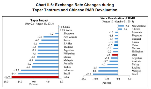 Typically, narrowing of yield differentials vis-à-vis the US and increase in stock market volatility embodied in the VIX have caused accentuation of exchange market pressures, including during the high intensity Chinese devaluation alluded to earlier (Charts II.7). Pressure on the exchange rate and on stock prices, accordingly, show an unusual degree of co-existence (Chart II.8). Prudential regulations in the form of capital and provisioning requirements for banks relating to unhedged forex exposures of their corporate clients nevertheless work to minimise balance sheet risks. 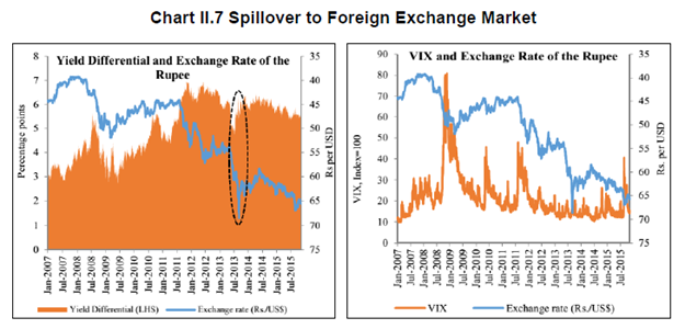
 Several EMEs face the compulsion of keeping their interest rates lower than what might have been warranted by Taylor type rules on account of the accommodation of external developments in their policy reaction functions (BIS, 2014). By contrast, the Reserve Bank’s main instrument to smooth excessive exchange rate volatility has been active capital account management along with interventions in the foreign exchange market (Mohan and Kapur, 2009). Since the early 2000s, there is no evidence of any systematic policy rate responses to exchange rate movements (Hutchison et al., 2010) except during the global financial crisis and the taper caper. Furthermore, the introduction of the Fed funds rate generates instability in the reaction function - the long-run coefficient on inflation falls below unity, while the coefficient on the output gap turns insignificant (Patra and Kapur, 2010). III. Measuring Spillovers on Global Financial Conditions Unconventional monetary policies (UMPs) have produced strong co-movements in a host of economic and financial variables across borders. In order to examine spillovers in relation to a specific country context, however, elements driving these co-movements must be identified and aggregated to uniquely represent an indicator of global spillovers (IGS). It has been empirically shown, that one or two common factors extracted from these innumerable variables may effectively capture a reasonably large part of the common information contained in them while maximising degrees of freedom (Breitung et al., 2006). Accordingly, dynamic factor models (DFMs) have been favoured for extracting latent dynamic factors in co-movements and synchronisations represented in high dimensional vectors of time series variables. DFMs overcome the limitations of standard VAR/GVAR approaches – restrictive assumptions on the structure of the economy; which variables to include and therefore, the number of shocks; difficulties in segregating global and country-specific factors; limitations in inclusion of number of countries; and the like (Giannone et al., 2004; Watson, 2004; Crucini, Kose and Otrok, 2011; Hirata, Kose and Otrok, 2013). Originating in seminal work on time series extensions of factor models developed for cross-sectional data (Geweke, 1977; Sargent and Sims, 1977), DFMs are able to simultaneously model data sets in which the number of variables can exceed the number of time series observations (Stock and Watson, 2011). Another advantage is that idiosyncratic movements from measurement errors or localised shocks can be eliminated, yielding more reliable policy signals (Breitung and Eickmeier, 2006). A similar parsimonious philosophy has driven the quest for financial conditions indices (Matheson, 2012; Osorio et al., 2011). A three-step procedure is adopted here. First, the extensive application of DFMs in the context of equity, bond and foreign exchange markets sheds light on the variables that are likely candidates for measuring global spillovers9: (i) VIX, as an indicator of risk perception or the confidence channel, exhibits strong co-movement with capital flows to EMEs in the role of a push factor (Nier et al., 2014); (ii) LIBOR-OIS spread as an indicator of the liquidity channel reflects US dollar liquidity stress (Ree and Choi, 2014) as well as risk of default associated with lending to other banks (Thornton, 2009); (iii) term spread, i.e., 10 year US Treasury yields minus three-month US treasury yields represents the portfolio balance channel (Bernanke, 2013)10; (iv) risk spread – US 10 year corporate yields minus US 10 year treasury yields (Bethke et al., 2015; Jaramillo and Weber, 2013b); and (v) DXY – the dollar index – represents the exchange rate channel of transmission of spillovers (Glick and Leduc, 2013; Bergsten, 2013). Hereafter, these variables are referred to as the spillover variables. In the second step, these variables are subjected to the Occam’s razor of being relevant to channels of transmission of monetary policy in India - the money market (spread between weighted average call rate and policy repo rate, with net injection/absorption of liquidity by the RBI as to control for market specific characteristics); the government bond market (10 year yield, with foreign portfolio investments in debt securities as the control variable); the stock market (BSE Sensex returns, with foreign portfolio equity investment as the control variable); and the foreign exchange market (returns on or daily change in the INR-USD exchange rate, with net FII investment - debt and equity together - as the control variable). For each domestic market segment, the relevant spillover variable is considered - LIBOR-OIS spread for the money market; the US term spread/risk spread for the bond market; the US VIX for the stock market; and LIBOR-OIS spread/DDXY (dollar index returns) for the foreign exchange market. These domestic market variables are hereafter referred to as domestic variables. Each postulated relationship is evaluated in a bivariate Baba, Engle, Kraft and Kroner (BEKK)-GARCH model11 (Engle and Kroner (1995) which involves a system of conditional mean equations with exogenous regressors in VARX(p, q) form: For the conditional variance equation, we also use a BEKK framework augmented with the spillover variables in view of the associated advantages of estimating less number of parameters and ensuring positive semi-definiteness of the conditional variance matrix. The equation takes the following form: in which Ht is a linear function of its own lagged values, lagged squared innovations (εt-1) and their cross-product, and exogenous spillover variables. Volatility transmission between domestic financial variables is represented by the off-diagonal parameters in matrices A and G while the diagonal parameters in those matrices capture the effects of their own past shocks and volatility. The parameters in matrix D measure international spillovers. (2) is estimated by the maximum likelihood method. Daily data for the period April 1, 2004 through October 15, 2015 are used, with estimations for the full sample period as well as for sub-samples covering the pre-crisis period (up to August 9, 2007) and the post-crisis period (from August 10, 2007 to October 15, 2015) as robustness checks. Impulse responses of the spillover variables on domestic variables in the unconditional VARX(p,q) models are found to be statistically significant though short-lived, with the impact persisting up to a maximum of one week (Appendix A, Charts). When examined in a conditional VAR framework that allows for interactions of volatilities in variance equations, the mean spillover effects are found to be only marginally different. Thus, even after controlling for interactions with volatility, there is evidence of spillover. Spillovers on to the call money market are found to be significant only in the post-crisis sample, essentially reflecting transient dollar liquidity shortages. Of the two spillover variables relevant for the foreign exchange market, the impact of the LIBOR-OIS spread on the exchange rate of the rupee is found to be significant - though at 10 per cent level - in the post-crisis period and the full sample period, though insignificant in the pre-crisis sub-sample. Importantly, spillover is found to transmit through FII flows, particularly in the post-crisis period. When the LIBOR-OIS spread is substituted with the DDXY, the impact is found to be significant in all sample periods, indicating that the rupee is directly influenced by movements of the US dollar vis-à-vis other major currencies. Mean spillovers on stock prices (daily returns) are found to be significant for the full sample as well as in the pre-crisis period; in the post crisis period, spillovers are more evident in stock price volatility rather than in mean returns. The mean spillover on government bond yields is found to be insignificant in all sample periods, though FII investments in debt are influenced by both term spread and risk spread. Turning to volatility, shocks to the LIBOR-OIS spread and the DXYSQ (i.e. squared dollar index return) are found to increase volatility in the exchange rate of the rupee in a statistically significant manner. Similar results are also obtained in the case of stock market volatility in response to shocks to the VIX, with a significantly large impact in the post-crisis period. The impact on volatility of bond yields is also statistically significant, but signs of coefficients reverse when the risk spread is considered, making the interpretation of the impact on mean and volatility difficult. An increase in the LIBOR-OIS spread is found to increase volatility in the call rate, despite the fact that net LAF liquidity - which should control both mean and volatility - is introduced in the model as a control variable. Overall, the five selected global spillover variables are found to influence volatility in domestic financial markets, and their effects on mean levels of variables are found to be statistically significant but transitory12. In the third stage, we estimate the IGS by applying a DFM to the selected spillover variables. It is assumed that each variable (standardized) Yt, can be decomposed into an unobserved common component, Ft, and a disturbance term εt. Ft is modeled as an autoregressive process and the disturbance term εt is assumed to be autocorrelated: Before estimation, all five spillover variables were converted to monthly frequency13 and standardised. The sample period for the analysis is from January 2002 to September 2015. The parameters are obtained by maximum likelihood estimation using Kalman filter (Appendix A) which produces substantial improvements in the estimates of factors relative to principal components when the common factor is persistent (Stock and Watson, 2011). The estimated factor loadings14 are provided in Table 1. | Table 1: Factor Loadings – GFC | | Variables | Factor Loadings | | VIX | 0.44 (0.00) | | LIBOR-OIS | 0.30 (0.00) | | DXYSQ | 0.15 (0.00) | | TMSPREAD | 0.01 (0.97) | | RISKSPREAD | 0.16 (0.00) | | (p-values are in brackets) | The Portmanteau (Q) test suggests that all innovations are white noise, validating the goodness of fit of the DFM. The indicator GFC is significantly correlated with all five spillover variables (Table 2), and especially with the VIX even when the other factors are taken into account. This result is consistent with the central tendency in the empirical literature (Nier et al., 2014). | Table 2: Correlation – IGS Indicator with Variables | | Variables | Correlation | | VIX | 0.99 (0.00) | | LIBOR-OIS | 0.74 (0.00) | | DXYSQ | 0.34 (0.00) | | TMSPREAD | 0.35 (0.00) | | RISKSPREAD | 0.67 (0.00) | | (p-values are in brackets) | IGS tracks global financial conditions nicely, particularly the global financial crisis, the events relating to UMPs of the Fed, the sovereign debt crisis in Europe, the Chinese devaluation, the bund tantrum and the growing certainty around the Fed’s lift off (Chart III.1). It does not, however, adequately capture the impact of the 2013 taper tantrum. Capital flows to EMEs reversed between May 2013 to January 2014, but recovered across all major EMEs by Q1 of 2014. This short-lived episode was also suffused with domestic policy responses in a number of countries, some dramatic and unconventional, which might be blurring the clear indications reflected in US yield spreads (see section II). Section IV: Impact of Spillovers on Transmission Channels in India In this section, we set out to empirically evaluate the hypotheses proposed in the introductory section, armed with the lessons drawn from the literature and the specifics of the Indian experience. With the failure of large macroeconometric models in predicting turning points of business cycles the world over, especially after the stagflation experience following the oil price shocks of the 1970s, economists turned to the use of vector autoregression (VAR) models, drawing on seminal work to capture the dynamics in multiple time series (Sims, 1980). While the VAR model has the advantage of being free of a priori strong commitment to structural restrictions, the imposition of constancy in parameters as well as error variances may produce misleading results, especially when policy reaction functions and transmission are changing either due to structural breaks/regime shifts and/or the changing nature of shocks. This is particularly relevant in the context of the period of study of this paper which covers a catastrophe of global dimensions and aftershocks as well as significant structural transformation in the Indian economy. These developments can and have forced changes in monetary policy transmission due to: (a) unconventional policy responses despite a stated objective function, leading to excessive accommodation/contraction, depending on the compulsion faced by central banks; and (b) exogenous non-policy factors influencing transmission such as asset quality concerns in the banking system and associated risk aversion, competition from non-banks/shadow banks, administered interventions in setting interest rates and macro-prudential and regulatory interventions impacting flow and pricing of credit. Accordingly, the methodology adopted here draws upon a recently growing strand in the literature which employs VAR models involving time-varying parameters (TVP) with stochastic volatility in the tradition started by Primiceri (2005); other important contributions are Cogley et al., 2008; Nakajima et al., 2011, Nakajima, 2011; Mumtaz and Plassmann, 2013; and John, 2015. The TVP-VAR also allows for the checking of impulse responses at different points of time. Following Imam (2015), the estimated cumulative impulse responses from the TVP-VAR – representing the impact of monetary policy shocks - are regressed on the IGS developed in Section III, while controlling for relevant domestic factors, in order to assess the impact of spillovers on monetary policy transmission in India. The interpretation of exogeneity in this context relates to non-policy factors, even though financial market variables included in the TVP-VAR reflect both policy and non-policy influences. The TVP-VAR Framework The measurement equation is specified as 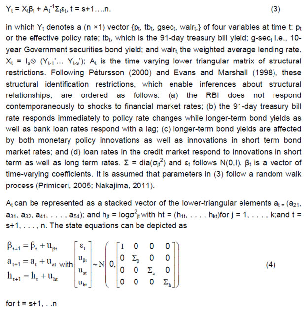 in which Σβ, Σa and Σh are the variance and covariance structure for the innovations of the time-varying parameters, and are assumed to be diagonal (Nakajima, 2011). Furthermore, a TVP-VAR requires somewhat tighter priors for the βs since the state variables capture both gradual and sudden changes in the underlying economic structure, which can lead to over-identification (Primiceri, 2005; Cogley et al. 2010 and Nakajima, 2011). Accordingly, a tighter prior is set for Σβ and a relatively diffuse prior for Σa and Σh. While the hyper-parameters of Σβ are simulated from an inverse Wishart distribution, the elements of Σa and Σh are drawn from an inverse gamma distribution. The prior density of ω = (Σβ, Σa, Σh) is π(ω). Samples of the posterior distribution π(β, a, h, ω|y) are drawn using a Bayesian Markov Chain Monte Carlo (MCMC) method. Due to lack of sufficient data points in the sample, we choose a reasonably flat prior for the initial state from the standpoint that we have no information about the initial state a priori. To compute15 the posterior estimates, 5,000 samples are drawn. The convergence diagnostics of the estimation results of the TVP-VAR model are provided in Appendix B which shows that the sample paths are stable. After the initial draws, the sample autocorrelations are low. Quarterly data from Q1: 1996-97 to Q2:2015-16 are used16. Results17 The accumulated time varying IRFs18 of monetary policy innovations for tbt, gsect, walrt exhibit sustained improvement in transmission over time, interrupted by spillover induced disruptions which produce short-lived overreactions to global event shocks. Nevertheless, monetary policy transmission has always been positive around a rising trend (Chart III.2). Transmission to 91-day T-Bill is almost complete and instantaneous in more recent years. Long term rates, i.e., the 10-year G-sec yield and the weighted average lending rate showed significant loss of traction to domestic monetary policy shocks during the financial crisis (2008-09), but transmission improved to pre-crisis levels and even strengthened till the taper tantrum. Long term rates overreacted to the exceptional monetary tightening in the second half of 2013, and corrected only gradually, showing up in a decline in the accumulated IRFs which still remained above pre-crisis levels. The estimated time-varying impulse response functions (IRFs) are presented in Chart B7, Appendix B. 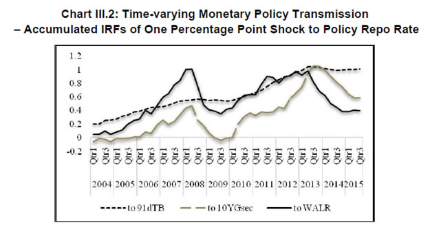 There are several market-specific idiosyncratic factors in operation which explain the time variation in the IRFs. Accordingly, the cumulative IRFs are regressed individually on the IGS while controlling for domestic market-specific factors - the size of the G-sec market in terms of volumes (G-sec volume/GDP) and inflation expectations - in the case of the 91-day T-Bill and 10 year G-sec yield IRFs. The Newey-West regression estimator is used to overcome autocorrelation and heteroskedasticity in the error term commonly associated with time series data, particularly, relating to financial markets. Given the need to identify the relative importance of each of the factors considered in the regression, standardized coefficients19 are reported in Table 3. Global spillovers (IGF) have a statistically significantly damping impact on monetary policy transmission to both G-Sec and 91-day T-Bill markets, but domestic factors such as volumes in the g-sec market and inflation expectations turned out to have a stronger influence20. As regards the bank lending rate, the IRF is regressed on IGS while controlling for financial developments in the credit market measured by credit to GDP ratio (credit/GDP) and asset quality measured by gross non-performing assets to credit ratio (GNPA/credit)21. The standardized regression coefficients on IGS are not statistically significant. By contrast, credit/GDP and GNPA/credit ratios are statistically significant and together explain more than 50 per cent of variations in transmission over time. Thus, there is no statistically strong evidence of domestic monetary policy losing traction in respect of bank lending rates because of spillovers. Table 3: Monetary Policy Transmission to G-Sec Markets
– Regression Estimates | | Dependent | Monetary Policy Transmission to | | Independent | 91 day T-Bill | G-Sec 10 year* | | Global spillover (IGS) | -0.274
(0.002) | -0.494
(0.013) | Market size
(G-sec volume/GDP) | 0.722
(0.000) | 0.680
(0.023) | | Long term Inflation Expectation | --- | 0.522
(0.011) | | R-squared | 0.548 | 0.422 | | F statistic | 28.40
(0.000) | 7.06
(0.001) | (p-values in brackets) Newey-West regression with autocorrelation & hetroscadasticity adjusted SEs.
*As the data on long-term inflation expectations are available from 2008, the sample period for this regression is from Q4:2007-08. |
Table 4: Monetary Policy Transmission to Credit Markets
– Regression Estimates | Dependent variable:
Monetary Policy
Transmission to WALR | Regression
1 | Regression
2 | Regression
3 | Regression
4 | | Global spillover (IGS) | -0.010
(0.912) | -0.011
(0.921) | -0.083
(0.473) | -0.010
(0.911) | | Financial development (credit/GDP) | 0.849
(0.000) | | | 0.775
(0.000) | | Asset quality (GNPA/credit) | | -0.732
(0.000) | | -0.087
(0.674) | Financial development*
Asset quality (or GNPA/GDP) | | | -0.512
(0.000) | | | R-square | 0.694 | 0.527 | 0.247 | 0.697 | | F statistic | 52.94
(0.000) | 27.74
(0.000) | 8.30
(0.000) | 34.81
(0.000) | | (p-values in brackets) Newey-West regression with autocorrelation and hetroscadasticity adjusted SEs | To summarise, the empirical results indicate that monetary policy transmission through the money market – the first leg of transmission – has improved substantially and is found to be almost complete even in the face of global spillovers. In the debt market, however, global spillovers affect transmission of monetary policy to yields and can even produce overshooting and over-corrections, but domestic factors such as market microstructure have a stronger influence. The latter may be influential in rendering the reactions to global perturbations short-lived and in ensuring mean reversions to normalcy. In the credit market, lending rates reflect low and incomplete transmission of monetary policy even absent global spillovers. Spillovers have no significant influence either; asset quality and financial deepening play the more important role in determining policy transmission. These findings do not, however, negate the overwhelming effects that global spillovers can produce on global output and inflation gaps and, in turn, on the domestic gaps. To that extent, spillovers do pose challenges to the successful conduct of monetary policy in pursuit of domestic goals. V. Conclusions The mainstream view that global spillovers overwhelm monetary policy independence is being questioned by specific country experiences. The focus of this ongoing debate is on the efficacy of monetary policy transmission, since the effects of UMPs on goal variables is still an unsettled issue. Here global real business cycles may be at work rather than financial forces. The arena shifts to the spectrum of financial markets which provide the transmission lines. In India, money markets are largely sheltered from spillovers, so too are credit markets, highlighting the shielding influence of the RBI’s active liquidity management, besides country specific factors that impart a distinct home bias. In bond, forex and equity markets in which foreign presence provides a conduit for contagion, capital flows management buffered by foreign exchange reserves will be tested for endurance in the period ahead by the exhaust fumes of Fed lift-off and the idling engines of monetary super accommodation. VAR and MGARCH estimates provide statistically significant evidence of spillovers transitorily affecting domestic financial markets. Extracting common elements in these spillovers through a dynamic factor model, a composite indicator of global spillovers (IGS) damps time varying monetary policy transmission in the domestic bond market. The credit market is impervious. In the money market, time varying transmission actually improves in times of global spillovers. Thus, there is no statistically strong evidence of domestic monetary policy losing traction. Monetary policy does respond directly to volatility-driven stress in domestic financial market conditions, but this needs to be regarded as a policy choice with the ultimate objective of meeting domestic goals, rather than a loss of monetary policy independence. Global shocks in a globalised economy are unavoidable, but stabilising the domestic economy irrespective of the nature and sources of shocks to domestic transmission channels remains a key task for domestic monetary policy.
References: Ahmed, S., Coulibaly, B. and Zlate, A. (2015). “International Financial Spillovers to Emerging Market Economies: How Important Are Economic Fundamentals?”, FRB International Finance Discussion Paper No. 1135. Aizenman, J. and Binici, M. (2015). “Exchange Market Pressure in OECD and Emerging Economies: Domestic vs. External Factors and Capital Flows in the Old and New Normal”, NBER Working No. 21662, October. Akram, T., and Das, A. (2015). “Does Keynesian Theory Explain Indian Government Bond Yields?”, Levy Economics Institute, Working Papers Series, No. 834. Amengual, D. and Watson, M. W. (2007). “Consistent estimation of the Number of Dynamic Factors in a Large N and T Panel”, Journal of Business and Economic Statistics, 25(1), 91-96. Atiyas, I., Bhorat, H., Derviş, K., Drysdale, P., Frischtak, C. R., Fujiwara, I., ... and Yu, Q. (2013). The G-20 and Central Banks in the New World of Unconventional Monetary Policy, Brookings, Washington, DC. Bacchetta, P. and Merrouche, O. (2015). “Global Financial Crisis and Foreign Currency Borrowing”, url: http://www.cepr.org/sites/default/files/Bacchetta-Final%20-%20Global%20Financial%20Crisis%20and%20Foreign%20Currency%20Borrowing _15032015.pdf Bai, J. and Ng, (2002). “Determining the Number of Factors in Approximate Factor Models”, Econometrica, 70(1), 191-221. ---- (2008). “Recent Developments in Large Dimensional Factor Analysis”, Working Paper, Mimeo. Bank for International Settlements (2014). Annual Report 2013/14, 29 June. Barroso, J. B., Kohlscheen, E. and Lima, E. J. (2014). “What have Central Banks in EMEs Learned About the International Transmission of Monetary Policy in Recent Years?”, BIS Papers No. 78, 95-109. Bellas, D., M. G. Papaioannou, and I. Petrova (2010). ‘‘Determinants of Emerging Market Sovereign Bond Spreads’’, in Braga, A. P. and Vincolette, C., Sovereign Debt and the Financial Crisis, The World Bank, Washington D.C., 77- 101. Bergsten, C. F. (2013). “Currency Wars, the Economy of the United States and Reform of the International Monetary System”, 12th Stavros Niarchos Foundation Lecture, Peterson Institute for International Economics. Bernanke, Ben S. (2013). “Long-Term Interest Rates”, Speech delivered at the Annual Monetary/Macroeconomics Conference: The Past and Future of Monetary Policy, March. Bethke, S., Gehde-Trapp, M. and Kempf, A. (2015). “Investor Sentiment, Flight-to-Quality, and Corporate Bond Comovement”, CFR Working Papers 13-06, University of Cologne. Bollerslev, T. and Engle, R.F., Wooldridge, J.M. (1988). “A Capital Asset Pricing Model with Time-Varying Covariance”, Journal of Political Economy, 96, 116–131. Breitung, J. and Eickmeier, S. (2006). “Dynamic Factor Models”, Allgemeines Statistisches Archiv, 90(1), 27-42. Bruno, V. and Shin, H. S. (2015). “Capital Flows and the Risk-taking Channel of Monetary Policy”, Journal of Monetary Economics, 71, 119-132. Brzoza-Brzezina, M., Chmielewski, T. and Niedźwiedzińska, J. (2010). “Substitution Between Domestic and Foreign Currency Loans in Central Europe, Do Central Banks Matter?”, ECB Working Paper Series, No 1187, May. Cerutti, E., Claessens, S. and Puy, M. D. (2015). “Push Factors and Capital Flows to Emerging Markets: Why Knowing Your Lender Matters More Than Fundamentals”, IMF Working Paper, No. 15-127, June. Chen, Q., Filardo, A., He, D. and Zhu, F. (2015). “Financial Crisis, US Unconventional Monetary Policy and International Spillovers”, BIS Working Papers, No. 494. Chua, W. S., Endut, N., Khadri, N. and Sim, W. H. (2013). “Global Monetary Easing: Spillovers and Lines of Defence”, Bank Negara Malaysia Working Paper Series, No. WP3/2013. Cogley, T., Primiceri, G. E. and Sargent, T. J. (2010). “Inflation-gap Persistence in the US”, American Economic Journal: Macroeconomics, 2(1), 43-69. Crucini, M. J., Kose, M. A. and Otrok, C. (2011). “What are the Driving Forces of International Business Cycles?”, Review of Economic Dynamics, 14(1), 156-175. Disyatat, P. and Rungcharoenkitkul, P. (2015). “Monetary Policy and Financial Spillovers: Losing Traction?” (No. 518). BIS Working Papers, No. 518. Edwards, S (2015): “Monetary Policy Independence under Flexible Exchange Rates: An Illusion?”, The World Economy, 38(5), 773-87. Eichengreen, B. and Gupta, P. (2014). “Tapering Talk: The Impact of Expectations of Reduced Federal Reserve Security Purchases on Emerging Markets”, World Bank Policy Research Working Paper, (6754). Eichengreen, B., Mody, A., Nedeljkovic, M. and Sarno, L. (2012). “How the Subprime Crisis Went Global: Evidence From Bank Credit Default Swap Spreads”, Journal of International Money and Finance, 31(5), 1299-1318. Engle, R. and Kroner, F.K. (1995), “Multivariate Simultaneous Generalized ARCH”, Econometric Theory, 11, 122–150. Evans, C. L. and Marshall, D. A. (1998). “Monetary Policy and The Term Structure of Nominal Interest Rates: Evidence and Theory”, in Carnegie-Rochester Conference Series on Public Policy, 49, North-Holland, 53-111. Feyen, E., Ghosh, S., Kibuuka, K. and Farazi, S. (2015). “Global Liquidity and External Bond Issuance in Emerging Markets and Developing Economies”, World Bank Policy Research Working Paper No. 7363. Geweke, J. (1976). “The Dynamic Factor Analysis of Economic Time Series Models”, in Aigner, D.J. and Goldberger, A.S. (ed.), Latent Variables in Socio-Economic Models, Amsterdam: North-Holland. Giannone, D., Reichlin, L. and Sala, L. (2004). “Monetary policy in Real Time”, in NBER Macroeconomics Annual 2004, Vol. 19, MIT Press, 161-224. Glick, R. and Leduc, S. (2013) “The Effects of Unconventional and Conventional US Monetary Policy on Dollar”, Working Paper 2013-11, Federal Reserve Bank of San Francisco. Gray, C (2013). ”Responding to a Monetary Superpower: Investigating the Behavioural Spillovers of US Monetary Policy”, Atlantic Economic Journal, 41(2), 173-84. Guo, K. and Stepanyan, V. (2011). “Determinants of Bank Credit in Emerging Market Economies”, IMF Working Papers, No. 11/51. He, D. and McCauley, R. N. (2013). “Transmitting Global Liquidity to East Asia: Policy Rates, Bond Yields, Currencies and Dollar Credit”, HKIMR Working Paper No.15. Hirata, H., Kose, M. A. and Otrok, C. (2013). “Globalization vs. Regionalization”, IMF Working Paper 13:19. Hofmann, B. and Takáts, E. (2015). “International Monetary Spillovers”, BIS Quarterly Review, September, 105-118. Hutchison, M., Sengupta, R. and Singh, N. (2010). “Estimating a Monetary Policy Rule for India”, Economic & Political Weekly, 45(38), 67-69. Imam, P. A. (2015). “Shock from Graying: Is the Demographic Shift Weakening Monetary Policy Effectiveness”, International Journal of Finance and Economics, 20(2), 138154. Jaramillo, L. and Weber, A. (2013a). “Bond Yields in Emerging Economies: It Matters What State You Are In”, Emerging Markets Review, 17, 169-185. ---- (2013b). “Global Spillovers into Domestic Bond Markets in Emerging Market Economies”, IMF Working Paper No. 13/264. John, J. (2015). “Has Inflation Persistence In India Changed Over Time?”, The Singapore Economic Review, 60(04), 1550095. Matheson, T. D. (2012). “Financial Conditions Indexes for the United States and Euro Area”, Economics Letters, 115(3), 441-446. Mesquita, M. and Torós, M. (2010). “Brazil and the 2008 Panic”, BIS Papers, No. 54, 113120. Mishra, P., Moriyama, K., N'Diaye, P. and Nguyen, L.(2014a). “Impact of Fed Tapering Announcements on Emerging Markets”, IMF Working Paper No. 14/109. Mishra, P., Montiel, P., Pedroni, P. and Spilimbergo, A. (2014b). “Monetary Policy and Bank Lending Rates in Low-income Countries: Heterogeneous Panel Estimates”, Journal of Development Economics, 111, 117-131. Miyajima, K., Mohanty, M. S., & Yetman, J. (2014). “Spillovers of US Unconventional Monetary Policy to Asia: the Role of Long-term Interest Rates”, BIS Working Paper No. 478. Mohan, R. and Kapur, M. (2009). “Managing the Impossible Trinity: Volatile Capital Flows and Indian Monetary Policy”, Working Paper No. 401, November, Stanford University. Mohanty, M and P Turner (2008). “Monetary Policy Transmission in Emerging Market Economies: What is New?”, BIS Papers, No 35, 1-59. Moreno, R. (2008). “Monetary Policy Transmission and the Long-term Interest Rate in Emerging Markets”, BIS Papers, No. 35, 61-80. ----- (2010). “Central Bank Instruments to Deal with the Effects of the Crisis on Emerging Market Economies”, BIS Papers, No. 54, 73-96. Moreno, R. and Villar, A. (2011). “Impact of the Crisis on Local Money and Debt Markets in Emerging Market Economies”, BIS Papers, No. 54, 49-72. Mumtaz, H. and Sunder‐Plassmann, L. (2013). “Time‐Varying Dynamics of the Real Exchange Rate: An Empirical Analysis”, Journal of Applied Econometrics, 28(3), 498-525. Nakajima, J. (2011). “Time-varying Parameter VAR Model with Stochastic Volatility: An Overview of Methodology and Empirical Applications”, Monetary and Economic Studies, November, 107-142. Nakajima, J., Kasuya, M. and Watanabe, T. (2011). “Bayesian Analysis of Time-varying Parameter Vector Autoregressive Model for the Japanese Economy and Monetary Policy”, Journal of the Japanese and International Economies, 25(3), 225-245. Nier, E. W., Saadi-Sedik, T. and Mondino, T. (2014). “Gross Private Capital Flows to Emerging Markets: Can the Global Financial Cycle Be Tamed?” IMF Working Paper No. 14/196. Obstfeld, M. (2015). “Trilemmas and Trade-offs: Living with Financial Globalisation”, BIS Working Paper No. 480. Osario, C., Unsal, D. F. and Pongsaparn, R. (2011). “A Quantitative Assessment of Financial Conditions in Asia”, IMF Working Papers, 1-21. Patra, M. and Kapur, M. (2010). “A Monetary Policy Model Without Money for India”, IMF Working Paper No. 10/183. Pattanaik, S. and Kavediya, R. (2015). “Taper Talk and the Rupee–Preconditions for the Success of an Interest Rate Defence of the Exchange Rate”, Prajnan, 44(3), 251-277. Pétursson, T. G. (2000). “The Representative Household's Demand for Money in a Cointegrated VAR Model”, The Econometrics Journal, 3(2), 162-176. Primiceri, G. E. (2005). “Time-Varying Structural Vector Autoregressions and Monetary Policy”, The Review of Economic Studies, 72(3), 821-852. Rajan, R.G. (2015). “India’s Central Bank Cuts Key Interest Rate More Than Expected”, Wall Street Journal, September 29. Ree, J. and Choi, S. (2014). “Safe-Haven Korea?: Spillover Effects from UMPs”, IMF Working Paper No. 14/53. Reserve Bank of India (2014). Annual Report 2013-14, August, Mumbai. ----- (2015). Annual Report 2014-15, August, Mumbai. Rey, H. (2015). “Dilemma not Trilemma: The Global Financial Cycle and Monetary Policy Independence”, NBER Working Paper No. 21162, May. Roley, V. V. and Sellon, G. H. (1995). “Monetary Policy Actions and Long-term Interest Rates”, Federal Reserve Bank of Kansas City Economic Quarterly, 80(4), 77-89. Saborowski, C. and Weber, S. (2013). “Assessing the Determinants of Interest Rate Transmission Through Conditional Impulse Response Functions”, IMF Working Paper No. 13/23. Sargent, T. J. and Sims, C. A. (1977). “Business Cycle Modeling Without Pretending to Have Too Much A Priori Economic Theory”, in Sims C. (ed), New Methods in Business Cycle Research, 1, Federal Reserve Bank of Minneapolis, 145-168. Shanmugaratnam, T. (2015). “Central Bankers Urge Fed to Get On With Interest-Rate Increase”, Wall Street Journal, October 11. Sims, C. A. (1980). “Macroeconomics and Reality”, Econometrica, 48 (1), 1-48. Singh, S. (2015). “Central Bankers Urge Fed to Get On With Interest-Rate Increase”, Wall Street Journal, October 11. Sobrun, J. and Turner, P. (2015). “Bond Markets and Monetary Policy Dilemmas for the Emerging Markets”, BIS Working Papers, No. 508. Stock, J. H. and Watson, M. W. (2006). “Forecasting with Many Predictors” in Elliott G., Granger C.W.J. and Timmermann A. (eds.), Handbook of Economic Forecasting, 1, North-Holland, Amsterdam 515-554. ---- (2011). “Dynamic Factor Models”, Oxford Handbook of Economic Forecasting, 1, 35-59. Takáts, E and A Vela (2014). “International Monetary Policy Transmission”, BIS Papers, .No 78, 25-44. Thornton, D.L. (2009) “What the LIBOR-OIS Spread Says”, Economic Synopses, No. 24, Federal Reserve Bank of St. Louis. Turner, P. (2014). “The Global Long-term interest rate, Financial Risks and Policy Choices in EMEs”, BIS Working Papers, No. 441. Watson, M. W. (2004). “Comment on Giannone, Reichlin, and Sala”, NBER Macroeconomics Annual 2004, Vol. 19, MIT Press, 216-221. Weidmann, J. (2015). “Central Bankers Urge Fed to Get On With Interest-Rate Increase”, Wall Street Journal, October 11.
Appendix A 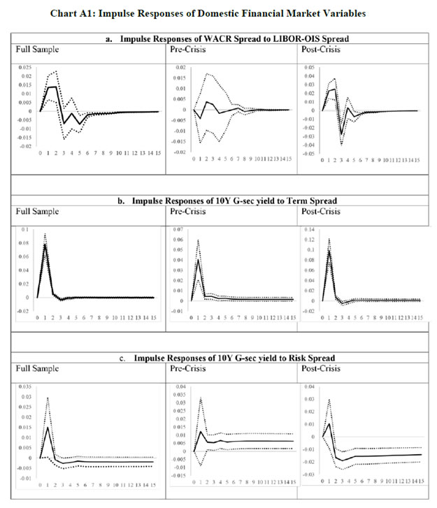
| Table A1: Spillover Impact in Money Market | | | Full Sample | Pre-Crisis | Post-Crisis | | | Mean Equation | | Dependent Variable: CALLSPREAD Constant | -0.27 | -(23.11)*** | -0.04 | -(2.74)** | -0.13 | -(6.78)*** | | CALLSPREADt-1 | 0.39 | (18.96)*** | 0.55 | (12.62)*** | 0.36 | (13.06)*** | | CALLSPREAD t-2 | 0.01 | (0.28) | 0.12 | (2.73)** | 0.06 | (1.98)** | | CALLSPREAD t-3 | 0.07 | (3.10)*** | 0.03 | (0.79) | 0.14 | (5.16)*** | | CALLSPREAD t-4 | 0.00 | (0.00) | 0.06 | (1.56) | 0.07 | (2.43)** | | CALLSPREAD t-5 | 0.08 | (3.88) *** | 0.08 | (2.66)** | 0.14 | (5.83)*** | | LAF t-1 | 0.00 | (9.41) *** | 0.00 | (4.36)*** | 0.00 | (5.99)*** | | LAF t-2 | 0.00 | (1.93)** | 0.00 | -(0.93) | 0.00 | (1.36) | | LAF t-3 | 0.00 | -(2.58)** | 0.00 | (0.00) | 0.00 | -(2.28)** | | LAF t-4 | 0.00 | -(0.34) | 0.00 | -(1.57) | 0.00 | -(0.72) | | LAF t-5 | 0.00 | -(0.69) | 0.00 | -(0.34) | 0.00 | (0.31) | | LIBOR_OIS t-1 | 0.00 | -(2.52)** | 0.00 | -(2.17)** | 0.00 | -(2.05)** | | Dependent Variable: LAF Constant | 0.52 | (0.21) | -5.18 | -(1.78)* | 21.25 | (3.40)*** | | CALLSPREADt-1 | 2.49 | (2.63)** | 1.63 | (1.65)* | -0.81 | -(0.16) | | CALLSPREAD t-2 | -0.36 | -(0.36) | 0.02 | (0.02) | 3.29 | (0.59) | | CALLSPREAD t-3 | -1.08 | -(1.00) | -1.46 | -(1.52) | -3.23 | -(0.54) | | CALLSPREAD t-4 | 0.57 | (0.53) | 0.85 | (0.88) | 9.62 | (1.79)* | | CALLSPREAD t-5 | -0.31 | -(0.33) | -0.74 | -(0.88) | 3.26 | (0.67) | | LAF t-1 | 0.94 | (48.90)*** | 0.97 | (32.69)*** | 0.99 | (41.70)*** | | LAF t-2 | -0.02 | -(0.74) | -0.07 | -(1.81)* | -0.04 | -(1.22) | | LAF t-3 | -0.07 | -(2.63)** | 0.00 | (0.05) | -0.12 | -(3.67)*** | | LAF t-4 | 0.02 | (0.71) | -0.03 | -(0.90) | 0.00 | (0.11) | | LAF t-5 | 0.11 | (5.94)*** | 0.09 | (3.42) *** | 0.15 | (6.57)*** | | LIBOR_OIS t-1 | -0.06 | -(0.80) | 0.09 | (0.65) | -0.25 | -(2.64)** | | | Variance Equation | | A{1}(1,1) | 0.56 | (17.23)*** | 0.76 | (11.06)*** | 0.70 | (20.83)*** | | A{1}(1,2) | 0.49 | (0.39) | 2.83 | (2.12)** | -5.91 | -(0.78) | | A{1}(2,1) | -0.00002 | -(0.14) | -0.002 | -(7.31)*** | 0.0004 | (6.52)*** | | A{1}(2,2) | 0.27 | (11.15)*** | 0.05 | (1.00) | 0.20 | (6.48)*** | | A{2}(1,1) | 0.69 | (17.80)*** | 0.45 | (5.60)*** | 0.50 | (8.43)*** | | A{2}(1,2) | 3.18 | (1.84)* | 1.22 | (1.06) | 47.99 | (4.45)*** | | A{2}(2,1) | -0.001 | -(10.24)*** | -0.001 | -(2.73)** | -0.001 | -(7.59)*** | | A{2}(2,2) | 0.19 | (5.14)*** | 0.13 | (3.31)*** | 0.28 | (6.27)*** | | B{1}(1,1) | 0.43 | (6.59)*** | -0.06 | -(0.33) | -0.31 | -(3.86)*** | | B{1}(1,2) | 13.47 | (5.86)*** | 0.81 | (0.66) | 16.87 | (1.90)* | | B{1}(2,1) | 0.00 | -(5.36)*** | 0.00 | -(0.30) | 0.00 | -(2.01)** | | B{1}(2,2) | -0.91 | -(17.07)*** | -0.23 | -(1.40) | -0.60 | -(7.27) *** | | B{2}(1,1) | 0.59 | (16.16)*** | 0.59 | (16.73)*** | 0.57 | (11.54) *** | | B{2}(1,2) | 3.32 | (1.79)* | -0.61 | -(0.76) | 32.42 | (2.79)** | | B{2}(2,1) | 0.00 | -(1.34) | 0.00 | (0.20) | 0.00 | -(2.19)** | | B{2}(2,2) | 0.25 | (1.49) | 0.85 | (15.37)*** | -0.11 | -(0.83) | | LIBOR_OIS i, t-1 | 0.002 | (4.29)*** | -0.01 | -(8.59)*** | 0.002 | (5.95)*** | | LIBOR_OIS j, t-1 | 0.16 | (4.67)*** | 0.59 | (6.07) *** | -0.34 | -(2.73)** | | Maximum eigenvalue | 0.78 | | 0.77 | | 0.74 | | | MV-ARCH-Q(12) | 48.62 (0.45) | 59.32 (0.13) | 70.63 (0.18) | Note: LIBOR_OISi, t-1LIBOR_OISj, t-1 are the exogenous variables in variance equations of CALLSPREAD and LAF, respectively.
Figures in parentheses are t-statistics when they are placed after coefficients and p-value, in case of ARCH tests.
Constants in variance equation are not presented here to save space.
*,*,***: indicates significant at 10%, 5% and 1% levels, respectively. |
| Table A2.a: Spillover Impact in G-Sec Market | | | Full Sample | Pre-Crisis | Post-Crisis | | | Mean Equation | | Dependent Variable: IN10YGS Constant | 0.05 | (4.42) *** | 0.04 | (2.32) ** | 0.06 | (3.31) *** | | IN10YGS t-1 | 1.04 | (55.40) *** | 1.08 | (31.52) *** | 0.99 | (38.17) *** | | IN10YGS t-2 | -0.05 | -(2.46) ** | -0.09 | -(2.49) ** | -0.001 | -(0.04) | | NFIIDR t-1 | -0.00001 | -(0.11) | 0.00003 | (0.06) | 0.00002 | (0.23) | | NFIIDR t-2 | 0.00004 | (0.40) | 0.00036 | (0.73) | -0.00008 | -(0.71) | | TMSPREAD t-1 | 0.00124 | (1.59) | -0.00031 | -(0.17) | 0.00224 | (1.34) | | Dependent Variable: NFIIDR Constant | 1.26 | (3.73) *** | 0.45 | (1.43) | -2.16 | -(1.00) | | IN10YGS t-1 | 1.02 | (1.38) | -1.36 | -(2.10) ** | -1.04 | -(0.45) | | IN10YGS t-2 | -1.17 | -(1.58) | 1.31 | (2.03) ** | 1.45 | (0.62) | | NFIIDR t-1 | 0.27 | (11.41) *** | 0.18 | (4.07) *** | 0.30 | (9.91) *** | | NFIIDR t-2 | 0.02 | (0.71) | -0.01 | -(0.48) | 0.23 | (7.89) *** | | TMSPREAD t-1 | -0.19 | -(5.70) *** | -0.12 | -(3.62) *** | -0.14 | -(0.50) | | | Variance Equation | | A{1}(1,1) | 0.17 | (5.59) *** | 0.31 | (12.52) *** | 0.28 | (14.77) *** | | A{1}(1,2) | -8.12 | -(9.10) *** | -0.54 | -(0.29) | -3.04 | -(0.87) | | A{1}(2,1) | -0.0001 | -(0.73) | 0.00 | (3.70) *** | -0.0002 | -(1.46) | | A{1}(2,2) | 0.81 | (29.97) *** | 0.93 | (18.92) *** | 0.63 | (16.48) *** | | A{2}(1,1) | -0.40 | -(17.90) *** | | | | | | A{2}(1,2) | 2.02 | (1.63) * | | | | | | A{2}(2,1) | 0.00002 | (0.13) | | | | | | A{2}(2,2) | 0.10 | (1.31) | | | | | | B{1}(1,1) | -0.13 | -(1.72) * | -0.91 | -(89.38) *** | 0.95 | (172.86) *** | | B{1}(1,2) | 0.29 | (0.40) | 1.88 | (1.65) * | -3.46 | -(1.88) * | | B{1}(2,1) | -0.0001 | -(1.39) | 0.004 | (5.82) *** | 0.00004 | (0.38) | | B{1}(2,2) | 0.53 | (9.73) *** | 0.20 | (1.64) * | 0.64 | (12.12) *** | | B{2}(1,1) | -0.88 | -(62.09) *** | | | | | | B{2}(1,2) | 0.46 | (0.39) | | | | | | B{2}(2,1) | -0.0003 | -(1.90) * | | | | | | B{2}(2,2) | 0.59 | (14.27) *** | | | | | | TMSPREAD i, t-1 | -0.002 | -(6.52) *** | 0.01 | (11.29) *** | 0.003 | (5.36) *** | | TMSPREAD j, t-1 | 0.000 | (0.00) | -0.18 | -(5.50) *** | 0.08 | (0.32) | | Maximum eigenvalue | 0.66 | | 0.93 | | 0.99 | | | MV-ARCH-Q(12) | 32.17 (0.96) | 21.21 (0.99) | 19.74 (0.99) | Note: TMSPREADi, t-1TMSPREADj, t-1 are the exogenous variables in variance equations of IN10YGS and NFIIDR, respectively.
Figures in parentheses are t-statistics when they are placed after coefficients and p-value, in case of ARCH tests.
Constants in variance equation are not presented here to save space.
*,*,***: indicates significant at 10%, 5% and 1% levels, respectively. |
| Table A2.b: Spillover Impact in G-Sec Market | | | Full Sample | Pre-Crisis | Post-Crisis | | | Mean Equation | | Dependent Variable: IN10YGS Constant | 0.05 | (4.16) *** | 0.04 | (2.72) *** | 0.08 | (3.23) *** | | IN10YGS t-1 | 1.06 | (54.89) *** | 1.10 | (35.48) *** | 1.01 | (46.06) *** | | IN10YGS t-2 | -0.07 | -(3.39) *** | -0.10 | -(3.35) *** | -0.018 | -(0.81) | | NFIIDR t-1 | -0.00007 | -(0.62) | 0.0004 | (0.72) | -0.00005 | -(0.46) | | NFIIDR t-2 | 0.00007 | (0.69) | 0.0007 | (1.08) | -0.00006 | -(0.56) | | RISKSPREAD t-1 | 0.00376 | (1.91) * | -0.0006 | -(0.12) | 0.00062 | (0.11) | | Dependent Variable: NFIIDR Constant | -0.70 | -(1.58) | 0.09 | (0.34) | 5.37 | (1.79) * | | IN10YGS t-1 | 0.58 | (0.63) | -1.36 | -(2.25) ** | -2.96 | -(1.40) | | IN10YGS t-2 | -0.48 | -(0.52) | 1.40 | (2.31) ** | 2.86 | (1.37) | | NFIIDR t-1 | 0.21 | (8.82) *** | 0.23 | (5.24) *** | 0.30 | (10.30) *** | | NFIIDR t-2 | 0.06 | (2.40) ** | -0.05 | -(1.56) | 0.22 | (8.54) *** | | RISKSPREAD t-1 | -0.103 | -(0.82) | -0.386 | -(3.95) *** | -2.03 | -(3.12) *** | | | Variance Equation | | A{1}(1,1) | -0.19 | -(9.33) *** | 0.24 | (7.96) *** | 0.16 | (5.71) *** | | A{1}(1,2) | -1.62 | -(1.25) | 1.64 | (0.89) | -1.30 | -(0.47) | | A{1}(2,1) | -0.0001 | -(0.93) | 0.001 | (0.94) | -0.001 | -(4.14) *** | | A{1}(2,2) | 0.68 | (19.25) *** | 0.91 | (16.21) *** | 0.67 | (16.36) *** | | A{2}(1,1) | 0.37 | (16.73) *** | 0.49 | (13.63) *** | 0.29 | (13.62) *** | | A{2}(1,2) | 2.96 | (3.03) *** | -0.89 | -(0.77) | 1.33 | (0.38) | | A{2}(2,1) | -0.0001 | -(0.46) | -0.001 | -(0.90) | 0.0001 | (0.42) | | A{2}(2,2) | 0.20 | (1.85) * | -0.10 | -(0.70) | -0.15 | -(1.05) | | B{1}(1,1) | 0.05 | (0.61) | -0.01 | -(0.11) | 0.05 | (0.56) | | B{1}(1,2) | 2.59 | (2.66) *** | 0.88 | (1.05) | -18.19 | -(5.61) *** | | B{1}(2,1) | -0.0003 | -(2.14) ** | 0.0002 | (0.20) | -0.0001 | -(0.53) | | B{1}(2,2) | 0.77 | (44.84) *** | 0.40 | (4.33) *** | 0.45 | (4.05) *** | | B{2}(1,1) | 0.90 | (93.50) *** | 0.84 | (53.46) *** | -0.94 | -(131.65) *** | | B{2}(1,2) | -3.02 | -(3.22) *** | -2.39 | -(1.44) | 3.61 | (1.32) | | B{2}(2,1) | 0.0003 | (1.80) * | -0.002 | -(1.08) | -0.001 | -(4.47) *** | | B{2}(2,2) | 0.03 | (0.28) | -0.23 | -(2.81) *** | -0.36 | -(5.01) *** | | TMSPREAD i, t-1 | -0.004 | -(4.38) *** | 0.01 | (3.60) *** | -0.03 | -(7.48) *** | | TMSPREAD j, t-1 | -2.89 | -(14.51) *** | -0.39 | -(0.96) | -4.43 | -(5.80) *** | | Maximum eigenvalue | 0.49 | | 0.99 | | 0.99 | | | MV-ARCH-Q(12) | 15.23 (1.00) | 61.57 (0.10) | 24.66 (0.99) | Note: RISKSPREADi, t-1RISKSPREADj, t-1 are the exogenous variables in variance equations of IN10YGS and NFIIDR, respectively.
Figures in parentheses are t-statistics when they are placed after coefficients and p-value, in case of ARCH tests.
Constants in variance equation are not presented here to save space.
*,*,***: indicates significant at 10%, 5% and 1% levels, respectively. |
| Table A3.a: Spillover Impact in Foreign Exchange Market | | | Full Sample | Pre-Crisis | Post-Crisis | | | Mean Equation | | Dependent Variable: DINR Constant | 0.00 | -(0.39) | 0.00 | (0.21) | 0.00 | (0.34) | | DINR t-1 | 0.01 | (0.29) | -0.01 | -(0.18) | 0.01 | (0.48) | | DINR t-2 | -0.01 | -(0.72) | 0.02 | (0.73) | -0.04 | -(1.83) * | | DINR t-3 | -0.02 | -(1.32) | -0.06 | -(2.14) ** | -0.01 | -(0.55) | | DINR t-4 | 0.00 | (0.20) | -0.06 | -(1.88) * | 0.02 | (0.89) | | NFII t-1 | -0.01 | -(0.42) | -0.02 | -(0.45) | -0.01 | -(0.35) | | NFII t-2 | -0.07 | -(2.36) ** | -0.10 | -(1.90) * | -0.01 | -(0.30) | | NFII t-3 | -0.04 | -(1.40) | -0.08 | -(1.46) | -0.03 | -(0.89) | | NFII t-4 | 0.03 | (0.98) | 0.09 | (1.84) * | -0.03 | -(0.70) | | LIBOR_OIS t-1 | 0.00 | (1.65) * | 0.00 | -(0.16) | 0.00 | (1.71) * | | Dependent Variable: NFII Constant | 0.03 | (6.39) *** | 0.02 | (4.38) *** | 0.07 | (9.50) *** | | DINR t-1 | -0.06 | -(8.39) *** | -0.04 | -(2.96) *** | -0.07 | -(7.14) *** | | DINR t-2 | -0.02 | -(2.52) ** | -0.02 | -(1.33) | -0.03 | -(3.49) *** | | DINR t-3 | 0.00 | (0.08) | -0.01 | -(0.61) | -0.02 | -(2.01) ** | | DINR t-4 | -0.01 | -(0.97) | 0.00 | (0.29) | -0.02 | -(2.39) ** | | NFII t-1 | 0.25 | (10.53) *** | 0.33 | (10.21) *** | 0.29 | (10.31) *** | | NFII t-2 | 0.14 | (6.32) *** | 0.02 | (0.53) | 0.14 | (5.45) *** | | NFII t-3 | 0.09 | (4.25) *** | 0.12 | (3.52) *** | 0.09 | (3.93) *** | | NFII t-4 | 0.09 | (4.87) *** | 0.08 | (2.48) ** | 0.06 | (2.96) *** | | LIBOR_OIS t-1 | 0.00 | -(2.09) ** | 0.00 | -(1.72) * | 0.00 | -(3.56) *** | | | Variance Equation | | A(1,1) | 0.29 | (16.93) *** | 0.47 | (11.84) *** | 0.22 | (12.17) *** | | A(1,2) | 0.00 | -(0.30) | -0.01 | -(0.76) | 0.01 | (0.46) | | A(2,1) | -0.04 | -(2.22) ** | 0.00 | (0.01) | -0.08 | -(1.60) | | A(2,2) | 0.25 | (18.51) *** | 0.31 | (13.75) *** | 0.50 | (10.80) *** | | B(1,1) | 0.96 | (192.97) *** | -0.87 | -(34.35) *** | 0.97 | (165.32) *** | | B(1,2) | 0.00 | (0.61) | 0.09 | (3.82) *** | -0.02 | -(1.76) * | | B(2,1) | 0.01 | (1.30) | -0.50 | -(4.98) *** | 0.08 | (1.24) | | B(2,2) | 0.97 | (398.46) *** | 0.98 | (131.86) *** | 0.55 | (9.37) *** | | LIBOR_OIS i, t-1 | 0.00 | (2.41) ** | 0.00 | (3.38) *** | 0.00 | (2.68) *** | | LIBOR_OIS j, t-1 | 0.00 | (1.75) * | 0.00 | (0.00) | 0.00 | -(1.85) * | | Maximum eigenvalue | 0.99 | | 0.93 | | 0.98 | | | MV-ARCH-Q(12) | 41.44 (0.74) | 39.49 (0.80) | 33.61 (0.94) | Note: LIBOR_OISi, t-1LIBOR_OISj, t-1 are the exogenous variables in variance equations of DINR and NFII, respectively.
Figures in parentheses are t-statistics when they are placed after coefficients and p-value, in case of ARCH tests.
Constants in variance equation are not presented here to save space.
*,*,***: indicates significant at 10%, 5% and 1% levels, respectively. |
| Table A3.b: Spillover Impact in Foreign Exchange Market | | | Full Sample | Pre-Crisis | Post-Crisis | | | Mean Equation | | Dependent Variable: DINR Constant | 0.01 | (0.97) | 0.00 | (0.09) | 0.02 | (1.81) * | | DINR t-1 | -0.02 | -(1.15) | -0.03 | -(0.90) | -0.01 | -(0.29) | | DINR t-2 | -0.01 | -(0.59) | 0.03 | (1.13) | -0.04 | -(1.56) | | DINR t-3 | -0.02 | -(0.98) | -0.05 | -(1.85) * | -0.01 | -(0.45) | | DINR t-4 | 0.01 | (0.70) | -0.05 | -(1.70) * | 0.02 | (0.85) | | NFII t-1 | 0.00 | -(0.49) | 0.00 | -(0.59) | 0.00 | -(0.96) | | NFII t-2 | 0.00 | -(2.75) *** | 0.00 | -(1.99) | 0.00 | -(0.28) | | NFII t-3 | 0.00 | -(0.75) | 0.00 | -(2.17) ** | 0.00 | -(1.06) | | NFII t-4 | 0.00 | (1.51) | 0.00 | (1.91) * | 0.00 | -(0.86) | | DDXY t-1 | 0.09 | (7.94) *** | 0.08 | (5.15) *** | 0.07 | (3.11) *** | | Dependent Variable: NFII Constant | 23.50 | (7.45) *** | 13.40 | (4.04) *** | 51.79 | (8.75) *** | | DINR t-1 | -50.86 | -(7.21) *** | -29.88 | -(2.89) *** | -64.88 | -(6.54) *** | | DINR t-2 | -17.72 | -(2.50) ** | -7.93 | -(0.71) | -29.42 | -(2.81) *** | | DINR t-3 | -6.05 | -(1.00) | -1.82 | -(0.19) | -21.84 | -(2.09) ** | | DINR t-4 | -5.13 | -(0.82) | -0.17 | -(0.02) | -19.46 | -(1.90) * | | NFII t-1 | 0.26 | (11.55) *** | 0.33 | (9.97) *** | 0.30 | (10.27) *** | | NFII t-2 | 0.18 | (8.89) *** | 0.03 | (0.73) | 0.14 | (5.63) *** | | NFII t-3 | 0.06 | (3.02) *** | 0.13 | (3.94) *** | 0.10 | (5.37) *** | | NFII t-4 | 0.07 | (3.48) *** | 0.07 | (2.48) ** | 0.06 | (3.34) *** | | DDXY t-1 | -19.55 | -(3.40) *** | -4.29 | -(0.75) | -12.19 | -(1.16) | | | Variance Equation | | A(1,1) | 0.24 | (20.74) *** | 0.50 | (11.88) *** | 0.22 | (11.71) *** | | A(1,2) | -42.79 | -(5.19) *** | 7.47 | (0.69) | 17.11 | (0.70) | | A(2,1) | 0.00 | (0.70) | 0.00 | (0.46) | 0.00 | -(2.09) ** | | A(2,2) | 0.44 | (18.66) *** | 0.30 | (13.46) *** | 0.54 | (11.85) *** | | B(1,1) | 0.97 | (343.97) *** | 0.84 | (36.74) *** | 0.97 | (166.98) *** | | B(1,2) | 11.12 | (4.71) *** | -1.25 | -(0.29) | -19.63 | -(1.79) * | | B(2,1) | 0.00 | -(2.16) ** | 0.00 | -(2.73) *** | 0.00 | (2.21) ** | | B(2,2) | 0.91 | (98.95) *** | 0.96 | (169.98) *** | 0.52 | (9.03) *** | | DXYSQ i, t-1 | 0.04 | (3.98) *** | -0.13 | -(4.67) *** | 0.04 | (3.03) *** | | DXYSQ j, t-1 | -19.84 | -(2.87) *** | -17.14 | -(2.98) *** | -11.60 | -(1.07) | | Maximum eigenvalue | 0.99 | | 0.95 | | 0.98 | | | MV-ARCH-Q(12) | 46.96 (0.52) | 28.16 (0.99) | 34.50 (0.93) | Note: DXYSQi, t-1DXYSQj, t-1 are the exogenous variables in variance equations of DINR and NFII, respectively.
Figures in parentheses are t-statistics when they are placed after coefficients and p-value, in case of ARCH tests.
Constants in variance equation are not presented here to save space.
*,*,***: indicates significant at 10%, 5% and 1% levels, respectively. |
| Table A4: Spillover Impact in Stock Market | | | Full Sample | Pre-Crisis | Post-Crisis | | | Mean Equation | | Dependent Variable: DLSENX Constant | 0.23 | (3.55) *** | 0.79 | (5.17) *** | 0.13 | (1.90) * | | DLSENX t-1 | 0.05 | (2.45) ** | 0.04 | (1.18) | 0.03 | (1.53) | | DLSENX t-2 | -0.01 | -(0.65) | -0.08 | -(2.23) ** | -0.03 | -(1.11) | | DLSENX t-3 | 0.00 | -(0.11) | 0.01 | (0.21) | -0.03 | -(1.17) | | DLSENX t-4 | 0.02 | (0.91) | 0.01 | (0.26) | 0.006 | (0.26) | | NFIIEQ t-1 | 0.00 | -(0.58) | 0.00 | (0.58) | -0.0005 | -(0.20) | | NFIIEQ t-2 | 0.00 | (0.44) | 0.00 | (0.65) | -0.0023 | -(1.04) | | NFIIEQ t-3 | 0.00 | -(1.04) | -0.01 | -(1.22) | -0.0015 | -(0.65) | | NFIIEQ t-4 | 0.00 | -(1.12) | -0.01 | -(1.88) * | -0.0036 | -(1.51) | | VIX t-1 | -0.01 | -(2.44) ** | -0.04 | -(4.15) *** | -0.0033 | -(0.89) | | Dependent Variable: NFIIEQ Constant | 2.40 | (8.80) *** | 3.45 | (4.97) *** | 3.53 | (10.20) *** | | DLSENX t-1 | 0.59 | (6.59) *** | 0.27 | (3.10) *** | 0.60 | (6.24) *** | | DLSENX t-2 | 0.03 | (0.34) | -0.09 | -(1.08) | 0.15 | (1.69) * | | DLSENX t-3 | 0.02 | (0.28) | 0.06 | (0.74) | -0.14 | -(1.58) | | DLSENX t-4 | -0.09 | -(1.05) | -0.08 | -(0.99) | 0.07 | (0.75) | | NFIIEQ t-1 | 0.30 | (12.57) *** | 0.29 | (7.31) *** | 0.36 | (12.03) *** | | NFIIEQ t-2 | 0.13 | (4.90) *** | 0.03 | (0.78) | 0.04 | (1.25) | | NFIIEQ t-3 | 0.07 | (2.89) *** | 0.12 | (3.28) *** | 0.09 | (4.43) *** | | NFIIEQ t-4 | 0.11 | (5.22) *** | 0.07 | (2.13) ** | 0.07 | (3.86) *** | | VIX t-1 | -0.06 | -(5.81) *** | -0.19 | -(4.25) *** | -0.08 | -(8.12) *** | | | Variance Equation | | A(1,1) | 0.25 | (18.12) *** | 0.38 | (11.24) *** | -0.02 | -(0.99) | | A(1,2) | -0.19 | -(1.60) | -0.22 | -(2.58) ** | -0.06 | -(0.54) | | A(2,1) | -0.01 | -(4.20) *** | 0.00 | (0.17) | -0.01 | -(1.75) * | | A(2,2) | 0.70 | (18.31) *** | 0.48 | (14.69) *** | 0.75 | (17.35) *** | | B(1,1) | 0.94 | (138.82) *** | 0.86 | (31.51) *** | -0.16 | -(0.52) | | B(1,2) | 0.41 | (4.54) *** | 0.07 | (1.70) * | 0.10 | (0.28) | | B(2,1) | 0.01 | (4.81) *** | 0.01 | (1.74) * | 0.00 | -(0.07) | | B(2,2) | 0.60 | (11.20) *** | 0.88 | (75.45) *** | 0.39 | (8.86) *** | | VIX i, t-1 | 0.02 | (8.19) *** | 0.03 | (3.68) *** | 0.05 | (15.07) *** | | VIX j, t-1 | -0.04 | -(3.93) *** | -0.39 | -(13.24) *** | -0.18 | -(16.26) *** | | Maximum eigenvalue | 0.98 | | 0.99 | | 0.72 | | | MV-ARCH-Q(12) | 56.02 (0.20) | 39.51 (0.80) | 63.22 (0.21) | Note: VIXi, t-1VIXj, t-1 are the exogenous variables in variance equations of DLSENX and NFIIEQ, respectively.
Figures in parentheses are t-statistics when they are placed after coefficients and p-value, in case of ARCH tests.
Constants in variance equation are not presented here to save space.
*,*,***: indicates significant at 10%, 5% and 1% levels, respectively. |
| Table A5. Estimated Coefficients – Dynamic Factor Model | | | Coef. | SE | z | p-value | 95%CI | | | Autocorrelated Factor | Factor
Lag 1 |
0.890 |
0.036 |
24.700 |
0.000 |
0.819 |
0.960 | | | Factor Loadings | VIX
Factor |
0.444 |
0.042 |
10.450 |
0.000 |
0.361 |
0.527 | LIBOR-OIS
Factor |
0.301 |
0.040 |
7.520 |
0.000 |
0.223 |
0.379 | DXYSQ
Factor |
0.151 |
0.034 |
4.470 |
0.000 |
0.085 |
0.217 | TMSPREAD
Factor |
0.001 |
0.017 |
0.040 |
0.972 |
-0.032 |
0.034 | RISKSPREAD
Factor |
0.160 |
0.029 |
5.550 |
0.000 |
0.103 |
0.217 | | | Autocorrelated Residuals | VIX Residual
Lag1 |
0.720 |
0.403 |
1.790 |
0.074 |
-0.070 |
1.511 | LIBOR-OIS Residual
Lag1 |
0.786 |
0.049 |
16.140 |
0.000 |
0.690 |
0.881 | DXYSQ
Residual
Lag1 |
-0.020 |
0.079 |
-0.260 |
0.796 |
-0.174 |
0.134 | TMSPREAD Residual
Lag 1 |
0.975 |
0.015 |
63.850 |
0.000 |
0.945 |
1.004 | RISKSPREAD Residual
Lag 1 |
0.913 |
0.031 |
29.830 |
0.000 |
0.853 |
0.974 |
Table A6. Portmanteau Test for White Noise of Innovations
– Dynamic Factor Model | | Innovations | Portmanteau (Q) statistic | p-value | | VIX | 9.186 | 0.057 | | LIBOR-OIS | 0.755 | 0.944 | | DXYSQ | 5.727 | 0.221 | | TMSPREAD | 6.950 | 0.139 | | RISKSPREAD | 8.015 | 0.091 |
Appendix B
Table B1. Structural VAR – Without Controlling for IGS
– Lagrange Multiplier Test | | Lag | Chi-Sq | df | Sig. | | 1 | 13.143 | 16 | 0.662 | | 2 | 16.095 | 16 | 0.446 | | 3 | 12.352 | 16 | 0.719 | | 4 | 12.693 | 16 | 0.695 | | 5 | 13.595 | 16 | 0.629 | | 6 | 14.026 | 16 | 0.597 | | 7 | 15.899 | 16 | 0.460 | | 8 | 25.349 | 16 | 0.064 |
| Table B2. Structural VAR – Controlling for IGS – Lagrange Multiplier Test | | Lag | Chi-Sq | df | Sig. | | 1 | 12.503 | 16 | 0.709 | | 2 | 22.037 | 16 | 0.142 | | 3 | 14.355 | 16 | 0.572 | | 4 | 17.619 | 16 | 0.347 | | 5 | 13.020 | 16 | 0.671 | | 6 | 16.719 | 16 | 0.404 | | 7 | 13.581 | 16 | 0.630 | | 8 | 31.217 | 16 | 0.013 |
| Table B3. Estimation Results of Selected Parameters in the TVP-VAR Model22 | | Parameter | Mean | Stdev | 95%U | 95%L | Geweke | Inef. | | sb1 | 0.210 | 0.035 | 0.160 | 0.302 | 0.931 | 5.570 | | sb2 | 0.194 | 0.023 | 0.160 | 0.263 | 0.787 | 4.690 | | sa1 | 0.419 | 0.165 | 0.215 | 0.733 | 0.922 | 31.780 | | sa2 | 0.350 | 0.173 | 0.234 | 0.903 | 0.923 | 8.170 | | sh1 | 0.313 | 0.097 | 0.208 | 0.535 | 0.913 | 9.510 | | sh2 | 0.315 | 0.065 | 0.207 | 0.452 | 0.962 | 1.930 |
|