The Indian banking sector continued to remain robust with adequate capital and liquidity buffers, and steady improvement in asset quality. Macro stress test results showed that SCBs’ aggregate capital levels will continue to remain above the regulatory minimum, even under adverse stress scenarios. The NBFC sector remained robust with an improvement in asset quality alongside healthy capital and profitability ratios. Interconnectedness among different categories of financial entities, in terms of outstanding bilateral exposures, continued to grow. Introduction 2.1 The Indian financial sector remained resilient amid a challenging global environment. Banks and non-banking financial companies (NBFCs) continued to strengthen their balance sheets, supported by healthy capital ratios as well as comfortable liquidity buffers, and non-performing assets ratios at multi-decadal lows. Bank credit growth remained strong and continued to outpace deposit growth. Credit expansion by NBFCs moderated, especially in the industry and services sectors, while asset quality improved further. Stress test results reaffirmed the resilience of these institutions to withstand losses under adverse scenarios, and to maintain capital ratios well above the regulatory minimum, at aggregate level. Other segments of the financial sector, including asset management companies, clearing corporations, and the insurance sector, also remained sound. 2.2 This chapter presents stylised facts and analyses on the health of the domestic financial sector and stress tests conducted to assess the resilience of the financial system. Section II.1 outlines the performance of scheduled commercial banks (SCBs) in India through various parameters, viz., business mix; asset quality; credit concentration; earnings; profitability and capital adequacy. Results of macro stress tests, sensitivity analyses and bottom-up stress tests performed to assess the resilience of SCBs under adverse scenarios are also presented. Sections II.2 and II.3 describe the performance of UCBs and NBFCs, respectively, including results of stress tests performed on these entities. Sections II.4 and II.5 examine the soundness of mutual funds and clearing corporations, respectively. Section II.6 covers a detailed analysis of the network structure and connectivity of the Indian financial system as well as contagion analysis under stress scenarios. II.1 Scheduled Commercial Banks (SCBs)1 2 3 2.3 The consolidated balance sheet of SCBs continued to remain resilient, with ongoing improvement in asset quality and capital ratios, and comfortable liquidity buffers. Credit and deposit growth gained momentum during the second half of 2025-26. Net interest margins (NIMs) remained broadly stable during the financial year. Growth in earnings before provisions and tax (EBPT) moderated as the growth in other operating income lost some traction in March 2026 (Table 2.1). II.1.1 Deposit and Credit 2.4 Aggregate deposits of SCBs grew at 11.5 per cent y-o-y during 2025-26. Private sector banks (PVBs) and foreign banks (FBs) recorded a surge in deposit mobilisation (Chart 2.1 a). The growth in term deposits continued to outpace that of current and savings account deposits, indicating sustained preference for interest-bearing term deposits (Chart 2.1 b). 2.5 SCBs’ credit growth accelerated to 14.5 per cent y-o-y during 2025-26, with PSBs continuing to outpace PVBs (Chart 2.1 c). Among broad economic sectors, shares of lending to services and personal loans increased over the previous year, while the share of credit to industry moderated (Chart 2.1 d). Credit growth across all four major sectors increased in March 2026, indicative of broad-based strengthening of credit demand (Chart 2.1 e). A decomposition of aggregate credit growth reveals that personal loans and services loans continued to be the principal drivers of overall credit growth of SCBs (Chart 2.1 f). Within personal loans segment, all bank groups continued to record robust growth in the other personal loans category (Chart 2.1 g).
II.1.2 Asset Quality 2.6 Asset quality of SCBs improved further in March 2026, with GNPA ratio declining to a multi-decadal low level of 1.8 per cent. The improvement in asset quality was broad-based across bank groups (Chart 2.2 a and b). 2.7 The annual slippage ratio steadily moderated over the last four financial years to 1.2 per cent in 2025-26, driven by lower fresh accretions to impaired assets in PSBs and PVBs (Chart 2.2 c). 2.8 The provisioning coverage ratio (PCR) of SCBs remained broadly stable at 75.6 per cent, indicative of continued prudence in balance sheet management (Chart 2.2 d). Write-offs relative to gross non-performing assets (GNPAs), however, remained elevated during 2025-26, particularly in the case of PVBs and FBs (Chart 2.2 e).
II.1.3 Sectoral Asset Quality 2.9 Credit quality improved across all broad economic sectors. Agriculture, despite improvement, continued to exhibit the highest GNPA ratio of 5.1 per cent and accounted for the largest share in SCBs’ GNPAs at 37.2 per cent in March 2026 (Chart 2.3 a). Within industry sub-sectors and the personal loans category, asset quality broadly improved across all segments (Chart 2.3 b and c). II.1.4 Credit Quality of Large Borrowers4 2.10 The share of large borrowers in total credit of SCBs increased marginally to 44.5 per cent as at end March 2026, however their share in gross NPAs declined steadily (Chart 2.4 a). Asset quality of large borrowers improved across bank groups, with the aggregate GNPA ratio declining sequentially to 1.2 per cent as at end-March 2026 from 2.4 per cent as at end-September 2024 (Chart 2.4 b). The volume of SMA-0, SMA-25 loans contracted, while that of SMA-1 loans increased in March 2026 (Chart 2.4 c).
II.1.5 Earnings and Profitability 2.11 As monetary policy easing transmitted progressively through the banking system during 2025-26, both the cost of funds and the yield on assets declined sequentially across bank groups in a largely synchronised manner, leaving net interest margins (NIMs) broadly unchanged over the period (Chart 2.5 a, b and c). Nevertheless, supported by higher credit volumes, growth in net interest income (NII) of SCBs recorded a modest improvement of 4.0 per cent y-o-y in March 2026 (Chart 2.5 d). 2.12 Growth in other operating income, although remaining robust at 14.5 per cent, lost some momentum in the quarter ending March 2026, resulting in a moderation in the growth of EBPT (Chart 2.5 d). Profit after tax (PAT) of SCBs increased to ₹4,05,268 crore during 2025-26 from ₹3,78,163 crore a year ago, driven by sustained credit expansion, stable interest margins and robust growth in other operating income (Chart 2.5 e). 2.13 Profitability indicators, namely RoE and RoA, remained broadly stable at the system level. Across bank groups, however, some divergence was observed beneath the aggregate picture. PSBs recorded a marginal improvement in both ratios during H2:2025-26, whereas FBs witnessed some moderation in profitability ratios (Chart 2.5 f and g).
II.1.6 Capital Adequacy 2.14 SCBs replenished their capital buffers, recording multi-decadal high capital to risk-weighted assets ratio (CRAR) and common equity tier 1 (CET1) ratio of 17.7 per cent and 15.3 per cent, respectively, as at end March 2026 (Chart 2.6 a). Both PSBs and PVBs reported higher CRAR in March 2026. The increase in CRAR in March 2026 can be attributed to higher growth in capital relative to the growth in risk-weighted assets (RWAs) during this period (Chart 2.6 b). 2.15 The evolving composition of capital suggests that the increase in total capital was driven almost entirely by CET1 capital (constituting 86 per cent of total capital), underscoring the increasing stock of high-quality capital within the banking system (Chart 2.6 c). Beneath the aggregate expansion in credit, the growth in credit risk-weighted assets (which account for nearly 86 per cent of total RWA) was lower than overall credit growth during 2025-26 for the first time in three years (Chart 2.6 d). This indicates a broad-based shift towards lower risk-weighted credit exposures and an improving risk profile of incremental lending. 2.16 The overall Tier I leverage ratio increased marginally to 8.2 per cent as at end-March 2026 (Chart 2.6 e).
II.1.7 Liquidity 2.17 At the aggregate level, the liquidity coverage ratio (LCR)6 and net stable funding ratio (NSFR)7 of SCBs moderated to 124.2 per cent and 122.1 per cent, respectively, though all bank groups continued to maintain liquidity buffers well above the respective regulatory minimum levels (Chart 2.7 a and b). II.1.8 Resilience – Macro Stress Test 2.18 Macro stress test assesses the resilience of SCBs to adverse macroeconomic shocks. It attempts to project capital ratios of banks under a baseline and two adverse macro scenarios over a two-year horizon. While the baseline scenario was derived from the latest forecasted paths of the macroeconomic variables, the two adverse scenarios are hypothetically stringent stress scenarios8 (Chart 2.8). (i) Adverse Scenario 1: This scenario assumes further intensification of geopolitical risks, elevated energy prices and exchange rate pressures, leading to rise in domestic inflation and growth slowdown during 2026-27, followed by a gradual improvement in the situation during 2027-28. (ii) Adverse Scenario 2: This scenario assumes prolonged and more widespread geopolitical conflicts extending to 2027-28, leading to disruptions in domestic inflation and growth in both the years. 2.19 The macro stress test results suggest the resilience of SCBs to macroeconomic shocks. The aggregate CET1 capital ratio of the select 46 banks may decline from 15.2 per cent in March 2026 to 13.9 per cent by March 2028 under the baseline scenario. It may decrease to 11.6 per cent and 11.4 per cent under adverse scenarios 1 and 2, respectively. Nonetheless, all banks would continue to meet the minimum CET1 capital ratio requirement of 5.5 per cent under all the scenarios (Chart 2.9).
2.20 The aggregate CRAR of 46 major SCBs may decline from 17.5 per cent in March 2026 to 15.6 per cent by March 2028 under the baseline scenario. It may fall to 13.3 per cent and 13.0 per cent under adverse scenarios 1 and 2, respectively (Chart 2.10 a). At the bank level, no bank would breach the minimum CRAR requirement of 9 per cent under the baseline scenario, while one and two banks may fall below the requirement under adverse scenarios 1 and 2, respectively (Chart 2.10 b). 2.21 The aggregate GNPA ratio of 46 banks may edge up from 1.8 per cent in March 2026 to 1.9 per cent by March 2028 under the baseline scenario. It may rise to 3.8 per cent and 4.1 per cent under adverse scenarios 1 and 2, respectively (Chart 2.11).
II.1.9 Sensitivity Analysis9 2.22 In sensitivity analyses10, shocks are applied to single factors like GNPA ratio, interest rate, etc., one at a time. This sub-section presents the results of top-down sensitivity analyses to assess the resilience of SCBs towards simulated credit, interest rate, liquidity risks, etc. under various stress scenarios, based on data as at end March 2026. a. Credit Risk 2.23 The resilience of SCBs to credit risk was assessed under two assumed stress scenarios - (i) one standard deviation (SD)11 [Shock 1] and (ii) two SD [Shock 2] rise in the aggregate level GNPA ratio as of March 2026. 2.24 Under the more severe shock scenario, viz., Shock 2, where the aggregate GNPA ratio of 46 select SCBs is assumed to move up to 8.1 per cent, there would be depletion in the CRAR and CET1 capital ratios by 400 bps and 420 bps, respectively (Chart 2.12 a). However, both the capital ratios would remain well above the respective regulatory minimum levels. The resultant capital impairment at the system level could be 25.2 per cent. The results of reverse stress test showed that shocks of 4.4 SD and 5.9 SD increase on the aggregate GNPA ratio would be required to bring down the system-level CRAR and the CET1 capital ratio, respectively, below their respective regulatory minima. 2.25 At bank group level, stress tests indicated relatively higher depletion in the capital of PSBs as compared to PVBs and FBs (Chart 2.12 b). At bank level, four banks with a share of 12 per cent in total assets of SCBs, would breach the regulatory minimum level of CRAR under Shock 2 (Chart 2.12 c). b. Credit Concentration Risk 2.26 Stress tests on banks’ credit concentration showed that in the extreme scenario of the top three individual borrowers of respective banks defaulting, the system level GNPA ratio would rise by 340 bps, and consequently, the CRAR and CET1 ratios would fall by 80 bps and 90 bps, respectively (Chart 2.13 a). Similarly, if the top three group borrowers default, the GNPA ratio would rise by 510 bps, and the CRAR and CET1 ratios would decline by 120 and 130 bps, respectively (Chart 2.13 b). However, even under such extreme scenarios, all banks would be able to maintain their capital ratios above the respective regulatory minimum levels. 2.27 Considering the system-wide impact of the top borrowers, the concentration of the top hundred borrowers, measured by the CR-100 ratio12, rose further in March 2026, reversing the decreasing trend observed until September 2025. The credit concentration risk index (CCRI)13 also increased in the last two quarters, indicating a rise in concentration risk within the top 100 borrowers (Chart 2.14).
c. Sectoral Credit Risk 2.28 Sectoral credit risk of SCBs was assessed under two hypothetical stress scenarios - (i) one SD14 [Shock 1] and (ii) two SD [Shock 2] increase in GNPA ratios of the respective sectors as of March 2026. The results of stress tests indicate only a marginal impact of such shocks on the aggregate capital of SCBs, underscoring the resilience of the banking system to sector-specific credit risk (Table 2.2). d. Interest Rate Risk15 16 2.29 For the sample of 46 SCBs under assessment, the market value of investments subject to fair value increased to a new high of ₹24.1 lakh crore in March 2026 from ₹22.8 lakh crore in September 2025 (Chart 2.15). Over the same period, the shares of PSBs and PVBs in aggregate fair-valued portfolio moderated, whereas the share of FBs increased. | Table 2.2: Sensitivity Analysis – Industry Sub-Sector Level | | (Basis points, in descending order for top 10 most sensitive sub-sectors) | | Industry | Decline in CRAR (basis points) | | 1 SD Shock | 2 SD Shock | | Basic Metal and Metal Products | 9 | 18 | | Infrastructure - Energy | 6 | 12 | | All Engineering | 3 | 7 | | Infrastructure - Transport | 3 | 6 | | Textiles | 2 | 4 | | Construction | 1 | 3 | | Vehicles, Vehicle Parts and Transport Equipment | 1 | 3 | | Food Processing | 1 | 2 | | Chemicals | 1 | 2 | | Gems and Jewellery | 1 | 2 | Note: For a system of select 46 SCBs.
Sources: RBI Supervisory Returns; and RBI Staff Estimates. | 2.30 The sensitivity (PV0117) of the AFS portfolio of SCBs marginally increased at an aggregate level in March 2026, largely driven by increase in PV01 of FBs (Table 2.3). While both PSBs and PVBs have decreased their modified duration for AFS portfolio, the aggregate AFS portfolio value rose by 7.0 per cent over September 2025. Although both PSBs and PVBs have reduced the PV01 of their FVTPL (including HFT) portfolios, a sharp increase by FBs have led to an increase in the PV01 of SCBs in March 2026. PSBs and FBs have increased their modified duration, while PVBs have reduced theirs. However, an overall 13.0 per cent decline in the FVTPL portfolio value for PSBs have reduced their PV01 despite the increase in modified duration. | Table 2.3: PV01 of AFS and FVTPL (including HFT) Portfolios | | (₹ crore) | | | AFS Portfolio | FVTPL (including HFT) Portfolio | | | Sep-25 | Mar-26 | Sep-25 | Mar-26 | | PSBs | 246.4 | 248.0 | 85.7 | 84.7 | | PVBs | 95.5 | 70.9 | 86.9 | 73.0 | | FBs | 18.9 | 44.1 | 232.2 | 314.1 | | All SCBs | 360.8 | 363.0 | 404.8 | 471.9 | | Sources: Individual Bank Submissions; and RBI Staff Estimates. |
2.31 In a stress scenario of a parallel upward shift of the yield curve by 250 bps, the impact on the fair-valued portfolio and the interest rate derivatives portfolio would reduce the system level CRAR and CET1 ratio by 99 bps and 100 bps, respectively (Table 2.4). At bank level, CRARs of two foreign banks would fall below the regulatory minimum of 9 per cent. 2.32 All bank groups incurred losses on securities trading in the quarter ending March 2026. For PSBs and PVBs, profits from securities trading declined steadily over the preceding three quarters, before turning negative in March 2026 (Table 2.5). FBs, on the other hand, have recorded trading losses for four consecutive quarters. 2.33 In the HTM portfolio, both PSBs and PVBs continued to increase their holding of state government securities (SGS) while paring their holdings in central government securities (G-Sec) and other HTM-eligible securities. FBs continued to increase the share of other securities in their HTM portfolio (Chart 2.16). During the quarter ending March 2026, both G-Sec and SGS holdings in the HTM book exhibited unrealised losses (Chart 2.17). | Table 2.4: Interest Rate Risk – Impact of Stress Test on Bank-Groups | | (Shock: 250 basis points parallel upward shift of the INR yield curve) | | | PSBs | PVBs | FBs | All SCBs | | | AFS | FVTPL
(incl. HFT) | AFS | FVTPL
(incl. HFT) | AFS | FVTPL
(incl. HFT) | AFS | FVTPL
(incl. HFT) | | Modified Duration (year) | 3.2 | 4.1 | 1.5 | 2.6 | 1.4 | 8.3 | 2.4 | 5.4 | | Share in Total Investments (per cent) | 18.4 | 5.0 | 17.8 | 10.7 | 38.6 | 47.6 | 20.3 | 11.4 | | PV01 of Fair Valued Portfolio (AFS + FVTPL) | 332.7 | 144.0 | 358.1 | 834.8 | | PV01 of Interest Rate Derivatives Held for Trading | 1.3 | 2.6 | 53.1 | 57.0 | | PV01 of Interest Rate Derivatives Held as Hedges18 | 0.0 | 39.6 | 10.5 | 50.2 | | Impact of 250 bps parallel upward shift in the INR yield curve: | | Reduction in CRAR (bps) | 85 | 28 | 588 | 99 | | Reduction in CET1 (bps) | 86 | 28 | 593 | 100 | Note: Share of total investments has been computed excluding investment in associates, subsidiaries, and JVs.
Sources: Individual Bank Submissions; and RBI Staff Estimates. |
| Table 2.5: Other Operating Income – Profit/ (Loss) on Securities Trading | | (₹ crore) | | | Q4: 2024-25 | Q1: 2025-26 | Q2: 2025-26 | Q3: 2025-26 | Q4: 2025-26 | | PSBs | 12,245 | 15,026 | 12,076 | 10,124 | -158 | | | (16.1) | (20.3) | (16.4) | (13.1) | (-0.2) | | PVBs | 2,761 | 15,320 | 3,493 | 2,460 | -280 | | | (3.7) | (17.4) | (4.5) | (3.2) | (-0.4) | | FBs | 2,927 | -340 | -2,586 | -1,413 | -9,597 | | | (22.7) | (-2.0) | (-16.8) | (-11.6) | (-63.2) | Note: Figures in parentheses represent other operating income (OOI)- Profit/ (Loss) on securities trading as a percentage of net operating income.
Source: RBI Supervisory Returns; and RBI Staff Estimates. |
2.34 If a shock of 250 bps parallel upward shift in the yield curve is applied, the MTM impact on the HTM portfolio of banks would result in additional unrealised loss in the HTM book by 10.5 per cent of the HTM portfolio size (book value). 2.35 An assessment of the interest rate risk of banks19, using traditional gap analysis (TGA) for rate-sensitive global assets, liabilities and off-balance sheet items, estimates that for a 200 bps increase in interest rate, the earnings-at-risk (EAR) for PSBs and PVBs would be 14.7 per cent and 14.1 per cent of NII, respectively (Table 2.6). The impact would be lesser for FBs and SFBs. The impact of an interest rate rise on earnings would be positive for PSBs, PVBs and FBs as their cumulative gap20 at bank group level was positive. In the case of SFBs, the impact would be negative as their cumulative gap was negative for March 2026. 2.36 As per the duration gap analysis21 (DGA) of risk-sensitive global assets, liabilities and off-balance sheet items, the market value of equity (MVE) for PVBs, FBs and SFBs would fall (rise) from an upward (downward) movement in the interest rate, while the impact on PSBs would be positive (Table 2.7). The MVE of SFBs would be particularly weighed down by an interest rate rise. | Table 2.6: Earnings at Risk (EAR) – Traditional Gap Analysis (TGA) | | (per cent) | | Bank Group | Earnings at Risk (till one year) as Percentage of Net Interest Income (NII) | | 100 bps Increase | 200 bps Increase | | PSBs | 7.4 (6.5) | 14.7 (13.1) | | PVBs | 7.0 (5.7) | 14.1 (11.5) | | FBs | 2.0 (1.4) | 4.1 (2.8) | | SFBs | -0.5 (-0.6) | -1.0 (-1.2) | Note: Figures in parenthesis represent the same values as of September 2025.
Sources: RBI Supervisory Returns; and RBI Staff Estimates. |
| Table 2.7: Market Value of Equity (MVE) – Duration Gap Analysis (DGA) | | (per cent) | | Bank Group | Market Value of Equity (MVE) as a Percentage of Equity | | 100 bps Increase | 200 bps Increase | | PSBs | 1.6 (0.8) | 3.1 (1.7) | | PVBs | -0.5 (-1.3) | -0.9 (-2.7) | | FBs | -1.5 (-2.6) | -3.0 (-5.1) | | SFBs | -6.2 (-6.7) | -12.5 (-13.3) | Note: Figures in parentheses represent the values as of September 2025.
Sources: RBI Supervisory Returns; and RBI Staff Estimates. | e. Equity Price Risk 2.37 As banks have limited direct capital market exposures due to regulatory guidelines, any impact of a possible significant fall in equity market prices on banks’ CRAR is expected to remain modest. Stress test results indicate that under scenarios involving a drop of 25, 35 and 55 per cent in equity prices, the system-level CRAR would decline by 14 bps, 20 bps and 32 bps, respectively (Chart 2.18).
f. Liquidity Risk 2.38 Liquidity stress test attempts to assess the impact of plausible run on deposits, and increased demand for unutilised portions of committed credit and liquidity facilities on the liquidity positions of banks. The baseline scenario for the stress test applies weights to each cashflow component22 as prescribed by the RBI guidelines on LCR computation23. The two stress scenarios are designed by applying higher run-off rates to certain cash outflow components. 2.39 The results showed that the aggregate LCR of the select SCBs would fall from 123.7 per cent in the baseline scenario to 116.7 per cent in stress scenario 1 and further to 110.8 per cent in stress scenario 2 (Chart 2.19 a). Individually, under the more severe stress scenario 2, three banks would fail to meet the regulatory minimum LCR (Chart 2.19 b and c). Among bank groups, the impact is highest for PSBs (decline of 13.9 percentage points under stress scenario 2). II.1.10 Sensitivity Analysis of Small Finance Banks – Credit Risk 2.40 Credit risk sensitivity analysis of SFBs has been carried out separately under two stress scenarios analogous to those of SCBs. Under the severe stress scenario of a two SD increase in the GNPA ratio, the aggregate GNPA ratio of SFBs would move up by 380 bps, causing fall in CRAR and CET1 ratio by 170 bps and 180 bps, respectively. Despite the overall resilience of the sector, one bank would breach the regulatory minimum CRAR requirement (Chart 2.20 a and b).
II.1.11 Bottom-up Stress Tests: Derivatives Portfolio 2.41 A series of bottom-up stress tests (sensitivity analyses) was undertaken by select banks24 subjecting their derivatives portfolio, as of March 2026 to four different shocks, viz., two each based on interest rates and foreign exchange rates. 2.42 Most of the FBs maintained a net positive mark-to-market position (chargeable to P&L) as a proportion of CET1 capital in March 2026. In contrast, the MTM impact remained largely muted for PSBs and PVBs (Chart 2.21). 2.43 The results of the stress test revealed that the impact of interest rate shocks gauged in terms of change in the net MTM position, while slightly elevated in March 2026 over that in September 2025, is symmetric with regard to P&L impact for both interest rate shocks (Chart 2.22). As regards shocks in terms of the rupee exchange rate, the pay-off profile has become more asymmetric, with potential losses from appreciation increasing significantly, implying accumulation of long USD positions.
2.44 The income from the derivatives portfolio, which includes changes in net MTM positions and the realised income, has increased sharply for FBs during March 2026. As regards PSBs and PVBs, the contribution of the income from the derivatives portfolio to the net operating income (NOI) is relatively muted (Chart 2.23). II.1.12 Bottom-up Stress Tests: Credit, Market and Liquidity Risk 2.45 A suite of bottom-up stress tests (sensitivity analyses) was conducted by 37 select banks on their balance sheet position as at end-March 2026. The results corroborated the resilience of these banks to multiple types and magnitudes of shocks. All sample banks would be able to meet the regulatory minimum requirement of CRAR under various scenarios (Chart 2.24).
2.46 The bottom-up stress test for liquidity risk revealed that the liquid assets ratios25 of all the sample banks would remain positive under alternate scenarios, emphasising the adequacy of their HQLAs to withstand liquidity pressure from sudden and unexpected withdrawal of deposits. Under the scenario of a three per cent deposit runoff for five consecutive days, the average liquid asset ratios of the select banks would drop from 21.4 per cent to 11.0 per cent (Chart 2.25).
II.2 Primary (Urban) Cooperative Banks26 2.47 Credit extended by primary urban co-operative banks (UCBs)27 recorded a robust y-o-y growth of 9.6 per cent in March 2026, supported by improvement across both scheduled UCBs (SUCBs) and non-scheduled UCBs (NSUCBs) (Chart 2.26 a). 2.48 UCBs’ income profile reflected higher net interest income (NII) and other operating income in March 2026 compared to the preceding year (Chart 2.26 c). NII recorded a y-o-y growth of 2.4 per cent in March 2026, driven primarily by higher growth among NSUCBs (Chart 2.26 d). At the aggregate-level, NIM improved marginally in March 2026 over the previous half year; however, it remained below the level recorded a year ago (Chart 2.26 e). Profitability indicators moderated, with RoA and RoE declining to 0.6 per cent and 6.3 per cent, respectively, in March 2026 (Charts 2.26 f and 2.26 g). Across different tiers28 of UCBs, profitability ratios witnessed a decline compared to the previous year (Chart 2.26 h). 2.49 The GNPA and NNPA ratios of UCBs declined significantly in March 2026 compared to September 2025 (Chart 2.26 b). The improvement was observed across both SUCBs and NSUCBs. A similar trend in GNPA ratios was evident among large borrowers, who accounted for 22.7 per cent share of UCBs’ loan portfolio (Chart 2.26 i). The PCR also improved in March 2026, compared to its levels in both March 2025 and September 2025, driven primarily by NSUCBs (Chart 2.26 j). Across all tiers of UCBs, asset quality improved, with an increase in PCR in March 2026 over the previous year (Chart 2.26 k).
2.50 The capital adequacy position of UCBs remained robust, with CRAR stable at 17.7 per cent in March 2026. CRAR across various tiers of UCBs continued to remain above the regulatory minimum requirement, notwithstanding a marginal decline compared to September 2025 (Chart 2.26 l and m). II.2.1 Stress Testing 2.51 Stress tests were conducted on a select set of UCBs29 to assess credit risk (default risk and concentration risk), market risk (interest rate risk in trading book and banking book) and liquidity risk, based on their reported financial positions as at end-March 2026. 2.52 Under the severe stress scenarios of credit default risk, credit concentration risk and interest rate risk (trading book), the consolidated CRAR of the select UCBs would fall from the pre-shock level of 17.2 per cent to 15.6 per cent, 13.9 per cent and 16.0 per cent, respectively (Chart 2.27 a). A severe interest rate shock in the banking book would lower the consolidated NII by 8.0 per cent. Under the liquidity stress test, the consolidated cumulative liquidity mismatch in the 1–28 days’ time bucket was positive under all three stress scenarios. 2.53 The impact of severe stress scenario for credit risk on CRAR30 will be significant for one UCB under Tier 4 category. In the case of Tier 2 and Tier 3 UCBs, the impact of credit risk and credit concentration risk under severe stress scenarios would be significant. Further, three Tier 4 UCBs would fall short of capital requirement under the severe stress scenario for credit concentration risk (Chart 2.27 b and c).
2.54 None of the Tier 1 and Tier 4 UCBs would breach the regulatory thresholds on CRAR under the interest rate shock scenarios applied to their trading book or experience more than 20 per cent decline in NII in their banking books (Chart 2.27 d). Under the severe stress scenario for interest rate risk (trading book), 10 Tier 2 and 11 Tier 3 UCBs would fall short of the regulatory minimum CRAR. A few UCBs in Tier 2 and 3 would face a negative liquidity mismatch of more than 20 per cent in the 1–28 days’ time bucket under the severe stress scenario (Chart 2.27 e and f). II.3 Non-Banking Financial Companies (NBFCs)31 2.55 The aggregate credit growth of NBFCs (Upper and Middle Layers) decelerated to 16.6 per cent y-o-y in March 2026 (Chart 2.28 a). Across activity-based categories, credit growth moderated for both NBFCICCs and NBFC-IFCs. In contrast, credit growth of NBFC-MFIs turned positive and accelerated to 14.5 per cent y-o-y in March 2026 (Chart 2.28 b). Sector-wise, NBFCs’ credit growth accelerated in the agriculture and retail loan segments, while slowed down in industry and services sectors (Chart 2.28 c). Within retail loans, growth was primarily driven by gold loans and other retail loans, whereas vehicle/ auto loans witnessed a slowdown (Chart 2.28 e). 2.56 The NII growth y-o-y of NBFCs increased by 9.7 per cent in March 2026 (Chart 2.28f). Profitability also improved, as reflected in PAT growth of 11.8 per cent. Growth in NII and PAT was higher in the case of upper layer NBFCs.
2.57 Asset quality of NBFCs continued to improve across all major economic sectors (Chart 2.28 d). Within retail loans, GNPA ratios recorded a marginal uptick in the housing and education loan segments (Chart 2.28 e). 2.58 On the liquidity front, short-term liabilities as a percentage of total assets increased marginally (Chart 2.28 g). 2.59 For a common set32 of NBFCs, growth in credit by NBFC-UL remained broadly stable at 19.8 per cent. NBFC-ML witnessed a pickup in credit growth from 12.6 per cent in September 2025 to 14.4 per cent in March 2026 (Chart 2.29 a and b). 2.60 Across major sectors, credit extended by NBFC-UL was concentrated in the retail (62.2 per cent) and the services sectors (25.5 per cent); however, credit growth to these segments slowed as of March 2026 (Chart 2.29 c). In the case of NBFC-ML, the credit portfolio was mostly concentrated towards the industrial sector, which accounted for 61.7 per cent of total lending. Credit growth in this segment also slowed considerably (Chart 2.29 d). 2.61 Asset quality improved, with a steady decline in GNPA ratios for both upper and middle layer NBFCs (Chart 2.29 e and f). NBFC-ML continued to maintain a much higher PCR than NBFC-UL. At the sectoral level, asset quality across sectors with major share in GNPA improved in March 2026 (Chart 2.29 g and h). 2.62 Key profitability ratios and regulatory capital ratios remained healthy, despite witnessing a decline in March 2026 (Chart 2.29 i, j, k and l). 2.63 While the funding pattern of NBFCs at the aggregate level remained more or less similar to that a year ago, dependence on bank borrowings increased for both NBFC-UL and NBFC-ML in March 2026 compared to the previous year (Table 2.8). Debentures and CPs constitute the other major sources of borrowing for both NBFC-UL and NBFC-ML. Furthermore, NBFC-UL’s share of secured borrowings and NBFC-ML’s share of unsecured borrowings have both increased in March 2026, with the increase in the latter being more pronounced. | Table 2.8: NBFCs’ Sources of Funds | | (Per cent) | | Item Description | NBFC-UL | NBFC-ML | NBFC-(UL+ML) | | Mar-25 | Mar-26 | Mar-25 | Mar-26 | Mar-25 | Mar- 26 | | I. Share Capital, Reserves and Surplus | 18.6 | 19.4 | 24.5 | 22.4 | 22.8 | 21.5 | | II. Total Borrowings | 71.1 | 70.8 | 67.5 | 69.5 | 68.5 | 65.9 | | Of which: | | | | | | | | (i) Secured | 61.6 | 62.4 | 30.9 | 30.8 | 39.9 | 40.8 | | (ii) Unsecured | 9.5 | 8.4 | 36.5 | 38.7 | 28.7 | 29.1 | | (1) From banks | 33.8 | 34.5 | 26.4 | 28.5 | 28.6 | 30.4 | | (a) Borrowings (Secured + Unsecured) | 29.9 | 30.6 | 24.0 | 26.3 | 25.7 | 27.6 | | (b) Debentures subscribed | 3.2 | 3.2 | 2.1 | 2.0 | 2.4 | 2.4 | | (c) CPs subscribed | 0.8 | 0.6 | 0.2 | 0.2 | 0.4 | 0.4 | | (2) Debentures (excluding II(1)(b)) | 16.3 | 16.2 | 23.8 | 23.9 | 21.6 | 21.5 | | (3) Commercial paper excluding II(1)(c)) | 2.6 | 2.6 | 1.6 | 1.4 | 1.9 | 1.8 | | III. Public Deposits | 6.0 | 5.3 | 0.5 | 0.5 | 2.1 | 2.0 | | IV. Provisions | 2.8 | 3.0 | 2.9 | 2.6 | 2.9 | 2.7 | | V. Other Liabilities | 1.6 | 1.5 | 4.6 | 4.9 | 3.7 | 3.8 | | Total | 100 | 100 | 100 | 100 | 100 | 100 | | Sources: RBI Supervisory Returns; and RBI Staff Estimates. |
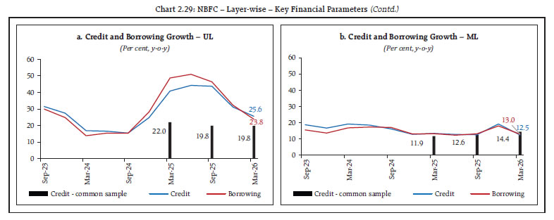
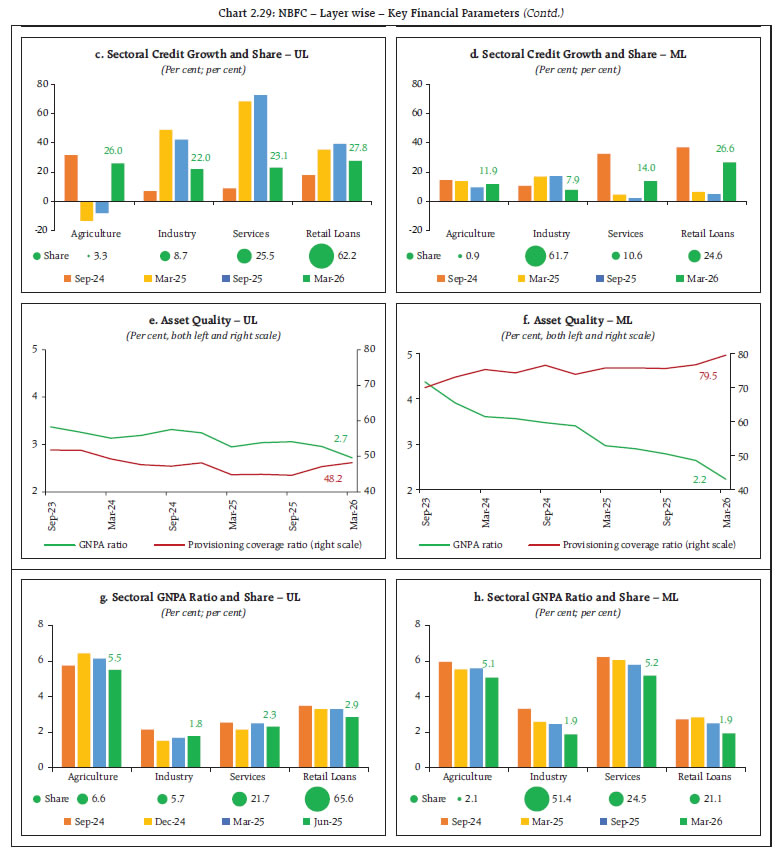
II.3.1 Stress Test33 – Credit Risk 2.64 System-level stress test was conducted on a sample of 174 NBFCs34 over a one-year horizon for assessing the resilience of the NBFC sector to credit risk shocks, under a baseline and two stress scenarios. While the baseline scenario was based on assumptions of business as usual, the medium and severe risk scenarios were derived by applying 1 SD and 2 SD shocks, respectively, to the GNPA ratio. 2.65 Under the baseline scenario, the system-level GNPA ratio of the sample NBFCs may rise from 2.4 per cent in March 2026 to 2.8 per cent in March 2027. Consequently, their aggregate CRAR may dip from 22.3 per cent to 20.8 per cent during the same period (Chart 2.30). Under the baseline scenario, 7 NBFCs may breach the minimum regulatory capital requirement of 15 per cent. Under the medium and severe stress scenarios, income loss and additional provision requirements may further reduce the aggregate CRAR by additional 60 bps and 80 bps, respectively, and 15 NBFCs may not be able to meet the regulatory minimum CRAR. 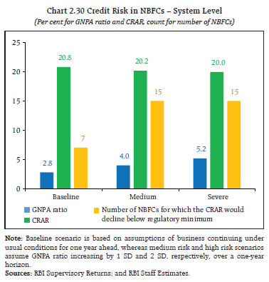 II.3.2 Stress Test35 – Concentration Risk 2.66 Stress test to assess NBFCs’ credit concentration risk showed that in the extreme scenario of the top three individual borrowers of respective NBFCs defaulting36, the system level CRAR would decline by 230 bps (Chart 2.31 a) and eight NBFCs would face a situation of a drop in CRAR below the regulatory minimum of 15 per cent. 2.67 Under the extreme scenario of the three group borrowers in the standard category failing to repay37, the system level CRAR would decline by 240 bps, and eight NBFCs would witness a drop in CRAR below the regulatory minimum of 15 per cent (Chart 2.31 b). II.3.3 Stress Test38 – Liquidity Risk 2.68 The resilience of the NBFC sector to liquidity shocks was assessed by estimating the impact of an assumed increase in cash outflows coupled with a decline in cash inflows39 on liquidity mismatch. The results revealed that the number of NBFCs which may experience a negative cumulative liquidity mismatch of over 20 per cent in the next one year would be two, five and six under the three scenarios, respectively (Table 2.9). II.4 Stress Testing of Mutual Funds40 2.69 Results of stress tests of mutual funds revealed that in March 2026, 44 open-ended debt schemes with total assets under management (AUM) of ₹3.18 lakh crore breached the AMFI or AMC prescribed thresholds (Table 2.10). In this respect, all the MFs have either cured the breach or reported initiation of remedial action and are expected to complete the same in the prescribed timeframe. 2.70 As part of liquidity risk management for open-ended debt schemes, two liquidity ratios, viz., redemption at risk (LR-RaR41) and conditional redemption at risk (LR-CRaR42) were computed by the top 10 AMCs (based on AUM) for 13 categories of open-ended debt schemes as at end of March 2026. Both the ratios were found well above the respective threshold limits for most of the MFs. A few instances of the ratios breaching the threshold limits were addressed by the respective AMCs in a timely manner (Chart 2.32). | Table 2.9: Liquidity Risk in NBFCs | | (Per cent) | | Cumulative Mismatch as Percentage of Outflows over the Next One Year | No. of NBFCs having Negative Mismatch | | Baseline | Medium | High | | Over 50 per cent | 1 (0.06) | 1 (0.06) | 1 (0.07) | | Between 20 to 50 per cent | 1 (0.77) | 4 (1.62) | 5 (1.83) | | Up to 20 per cent | 4 (1.06) | 21 (11.50) | 35 (17.69) | Note: Baseline scenario is based on projected outflows and inflows over the next one year; medium risk scenario assumes a 5 per cent decrease in inflows and a 5 per cent increase in outflows while high risk scenario assumes a 10 per cent decrease in inflows and a 10 per cent increase in outflows. Figures in parentheses represent percentage shares in the asset size of the sample.
Sources: RBI Supervisory Returns; and RBI Staff Estimates. |
| Table 2.10: Stress Testing of Open-Ended Debt Schemes of Mutual Funds – Summary Findings – March 2026 | | | Breach of Thresholds | No Breach of Thresholds | Total | | No. of AMCs | 28 | 14 | 42 | | No. of Schemes | 44* | 282 | 326 | | AUM (₹ lakh crore) | 3.18 | 13.07 | 16.25 | Note: * The number of schemes which breached the respective prescribed thresholds for interest rate risk, credit risk and liquidity risk are 22, 22 and seven, respectively, while the total number of unique schemes which breached any of the prescribed thresholds is 44.
Source: SEBI. |
2.71 Stress test results and liquidity analysis of midcap and smallcap equity schemes of AMCs showed that in April 2026, the number of days to liquidate 25 per cent of the portfolio for the top 5 schemes (in terms of AUM) ranged from 5 to 23 days for midcap schemes and 7 to 33 days for smallcap schemes (Table 2.11). II.5 Stress Testing Analysis at Clearing Corporations43 2.72 Stress testing has been carried out at clearing corporations (CCs) to determine the segment-wise minimum required corpus (MRC), which needs to be contributed by clearing members (CMs) to the core settlement guarantee fund (Core SGF). Stress test analysis for the period December 2025 to March 2026 indicated that the actual MRC requirement remained the same for most of the segments, except for the equity derivatives segment, wherein the actual requirement increased for Clearing Corporation 2 and for the commodity derivatives segment, wherein the actual requirement increased for Clearing Corporation 3 during the period (Table 2.12). II.6 Financial Network and Contagion Analysis 2.73 Interconnections among financial institutions arise from funding relationships, liquidity mismatches and maturity transformation, payment and settlement processes and risk transfer mechanisms. The financial system can be viewed as a network in which financial institutions act as nodes, while bilateral exposures among them serve as links connecting these nodes. These links could be in the form of loans to, investments in, or deposits with each other, which act as sources of funding, liquidity, investment and risk diversification. While these links enhance the efficiency and resilience of the financial system by improving resource allocation and diversifying risks, they can also become conduits of risk transmission and amplification in a crisis. Understanding the nuances of risk propagation through these networks is therefore useful for assessing systemic risk and devising appropriate policy responses to safeguard financial and macroeconomic stability. | Table 2.11: Summary of Stress Tests and Liquidity Analysis of MF Midcap and Smallcap Equity Schemes | | Schemes/Month | Midcap Schemes | Smallcap Schemes | | Dec-25 | Jan-26 | Feb-26 | Mar-26 | Apr-26 | Dec-25 | Jan-26 | Feb-26 | Mar-26 | Apr-26 | | No. of days to liquidate 25 per cent of portfolio-Range for top 5 schemes w.r.t. AUM | 5 to 21 | 5 to 27 | 4 to 28 | 4 to 25 | 5 to 23 | 11 to 44 | 12 to 51 | 12 to 43 | 13 to 38 | 7 to 33 | | Concentration-Asset Side | Largecap | 12.9 | 13.2 | 13.6 | 13.3 | 13.4 | 8.5 | 8.6 | 8.4 | 8.2 | 8.0 | | Midcap | 69.0 | 68.8 | 69.2 | 69.1 | 69.5 | 12.7 | 12.3 | 12.1 | 12.0 | 12.7 | | (AUM held in per cent) | Smallcap | 12.9 | 14.1 | 13.5 | 13.4 | 13.4 | 73.5 | 73.9 | 73.6 | 73.6 | 73.5 | | Cash | 5.1 | 3.9 | 3.6 | 4.2 | 3.7 | 5.4 | 5.2 | 5.9 | 6.0 | 5.8 | | Sources: AMFI. |
| Table 2.12: Minimum Required Corpus of Core SGF Based on Stress Testing Analysis at Clearing Corporations | | (₹ crore) | | Segment | Dec-25 | Jan-26 | Feb-26 | Mar-26 | Dec-25 | Jan-26 | Feb-26 | Mar-26 | | Clearing Corporation 1 | Average Stress Test Loss | Actual MRC Requirement | | Equity Cash Segment | 106 | 86 | 92 | 105 | 388 | 388 | 388 | 388 | | Equity Derivatives Segment | 9,243 | 8,871 | 7,196 | 5,918 | 10,500 | 10,500 | 10,500 | 10,500 | | Currency Derivatives Segment | 90 | 89 | 78 | 125 | 161 | 161 | 161 | 161 | | Debt Segment | - | - | - | - | 4 | 4 | 4 | 4 | | Tri-Party Repo Segment | - | - | - | - | 17 | 17 | 17 | 17 | | Commodity Derivatives Segment | 9 | 8 | 5 | 8 | 15 | 15 | 15 | 15 | | Total | 9,448 | 9,055 | 7,371 | 6,156 | 11,085 | 11,085 | 11,085 | 11,085 | | Clearing Corporation 2 | Average Stress Test Loss | Actual MRC Requirement | | Equity Cash Segment | 69 | 72 | 42 | 68 | 194 | 194 | 194 | 194 | | Equity Derivatives Segment | 715 | 707 | 712 | 618 | 723 | 733 | 733 | 733 | | Currency Derivatives Segment | 0 | 1 | 1 | 9 | 10 | 10 | 10 | 10 | | Debt Segment | 0 | 0 | 0 | 0 | 0 | 0 | 0 | 0 | | Tri-Party Repo Segment | 0 | 0 | 0 | 0 | 0 | 0 | 0 | 0 | | Commodity Derivatives Segment | 0 | 0 | 0 | 0 | 14 | 14 | 14 | 14 | | Total | 784 | 780 | 755 | 694 | 942 | 951 | 951 | 951 | | Clearing Corporation 3 | Average Stress Test Loss | Actual MRC Requirement | | Commodity Derivatives Segment | 749 | 1,046 | 1,248 | 804 | 990 | 990 | 990 | 1,046 | | Clearing Corporation 4 | Average Stress Test Loss | Actual MRC Requirement | | Commodity Derivatives Segment | 49 | 36 | 48 | 55 | 124 | 124 | 124 | 124 | Notes: Average Stress Test Loss calculated for a month M is applicable, as MRC, from the month M+2. SEBI, vide letter dated March 27, 2025, has permitted Clearing Corporations 1 and 2 for the resetting of Minimum Required Corpus (MRC) of the currency derivatives segment and subsequent transfer of funds to the Core SGF of the equity derivatives segment. Accordingly, MRC for the Core SGF of the currency derivatives segment has been reset based on the highest stress losses observed since May 2024, subject to a minimum threshold of ₹10 crore. Hence, there is a decrease in the MRC value for the currency derivatives segment for Clearing Corporation 1 from May 2025 onwards on account of reduced volumes in the currency derivatives segment.
Source: Clearing Corporations. | II.6.1 Financial System Network44 2.74 The network analysis covers 280 financial entities45. Total outstanding bilateral exposures46 of the 280 entities expanded by 20.1 per cent in March 2026 y-o-y. Of this, SCBs continued to hold the largest share (45.5 per cent) in the network, followed by NBFCs (18.5 per cent) and AIFIs (13.7 per cent) (Chart 2.33 a and b). 2.75 The interconnectedness of SCBs with NBFCs, HFCs, AIFIs and AMC-MFs remained strong. Among these groups, AIFIs were closely connected to SCBs through both asset and liability sides of their balance sheets (Chart 2.33 c). 2.76 Loans and advances, capital/ equity investments and long-term (LT) debt instruments remained the leading instruments of bilateral exposures within the financial network (Chart 2.34). Long-Term (LT) funding, which accounted for 59.8 per cent, continued to dominate the total bilateral exposures as of March 2026. Funding structures, however, witnessed some change during 2025-26, with the share of short-term (ST) deposits increasing, while those of equity investments, LT debt instruments and ST loans moderating. 2.77 In terms of inter-sectoral exposures47, AMC-MFs, insurance companies and PSBs continued to be the largest fund providers in the system, while NBFCs, PVBs and HFCs remained as net receivers of funds. Among bank groups, PSBs, UCBs and FBs held net receivable positions, whereas PVBs and SFBs held net payable positions (Chart 2.35). 2.78 The net receivable and net payable positions of various groups increased in March 2026 as compared to March 2025 (Chart 2.36 a). Net borrowing by NBFCs and private banks increased further between March 2025 and March 2026, indicating a rise in inter-institutional funding, while the net receivable positions of AMC-MFs and insurance companies also expanded correspondingly. In terms of shares in gross financial system exposure over time, net receivables/ payables across the financial system remained concentrated among a few major sectors, with AMC-MFs, insurance companies, PSBs and PFs continuing to be net providers of funds, while NBFCs, private banks and HFCs remained the largest net borrowers (Chart 2.36 b), while the total gross exposure across categories increased from ₹32.45 lakh crore in September 2018 to ₹93.2 lakh crore in March 2026.
a. Inter-Bank Market 2.79 Inter-bank exposures as a percentage of the total assets of the banking system edged up over the last two quarters and stood at 3.4 per cent. The increase was primarily driven by fund-based exposures48, while non-fund-based exposures49 remained broadly stable during the period (Chart 2.37 a). 2.80 PSBs continued to dominate in the inter-bank market, accounting for 57.8 per cent of total inter-bank exposures as at quarter ended March 2026, while the share of FBs witnessed a gradual increasing trend in the recent quarters (Chart 2.37 b). 2.81 The composition of short-term inter-bank funding underwent a modest shift during 2025-26, characterised by an increase in the share of ST deposits and a corresponding decline in CDs. ST deposits remained the dominant source of short-term funding, while ST loans continued to constitute the second largest component. The composition of long-term inter-bank funding continued to be dominated by LT loans and LT debt instruments, which together accounted for a major share of LT funds (Chart 2.38 a and b). b. Inter-Bank Market: Network Structure and Connectivity 2.82 The interconnectedness within the banking network (SCBs and SUCBs) remained skewed, with only a few SCBs (seen in the core and mid network) holding majority of the linkages, as reflected by the typical core-periphery network structure50 51. As of March 2026, five banks were in the inner-most core, and seven banks were in the mid-core circle, consisting of PSBs and PVBs. The periphery of the banking network was occupied mainly by FBs, UCBs and SFBs (Chart 2.39).
2.83 The connectivity ratio52, defined as the degree of interconnection among banks (SCBs and SUCBs), and the local interconnectedness in terms of the cluster coefficient53 decreased marginally at end-March 2026 (Chart 2.40). c. Exposure of AMC-MFs 2.84 Gross receivables of AMC-MFs, the largest fund providers, increased marginally to ₹23.95 lakh crore in March 2026, from ₹23.27 lakh crore in September 2025 (as reported in December 2025 FSR), against their gross payables of ₹1.46 lakh crore. SCBs (primarily PVBs) remained the major recipients of funds from AMC-MFs, followed by NBFCs, AIFIs and HFCs (Chart 2.41). d. Exposure of Insurance Companies 2.85 With gross receivables at ₹13.44 lakh crore against gross payables at ₹1.56 lakh crore, insurance companies were the second largest net providers of funds to the financial system as of March 2026. SCBs (primarily PVBs) were the largest recipients of their funds, followed by NBFCs and HFCs (Chart 2.42).
e. Exposure to NBFCs (Non-HFCs) 2.86 NBFCs (Non-HFCs) were the largest net borrowers of funds from the financial system, with higher gross payables at ₹26.57 lakh crore against gross receivables at ₹2.88 lakh crore as at end-March 2026. More than half of their funds continued to be sourced from SCBs, followed by insurance companies and AMC-MFs (Chart 2.43 a). LT loans and LT debt remained the preferred modes of funding for NBFCs (Non-HFCs) (Chart 2.43 b).
f. Exposure to HFCs 2.87 HFCs, the third largest net borrowers, had gross payables at ₹7.35 lakh crore against gross receivables of ₹0.19 lakh crore in March 2026. SCBs continued to be the largest providers of funds, with rising share, accompanied by a corresponding decrease in shares of funding from AMC-MFs and Insurance Companies. About 73.6 per cent of HFCs’ funds was sourced through LT loans and LT debt instruments (Chart 2.44 a and b). g. Exposure of AIFIs 2.88 With gross payables and receivables at ₹10.61 lakh crore and ₹9.71 lakh crore, respectively, AIFIs were both active borrowers and lenders in the financial system and had a net payable position of around ₹0.9 lakh crore in March 2026. While the AIFIs raised funds mainly from SCBs, AMC-MFs and insurance companies, they lend predominantly to SCBs (79.9 per cent in March 2026) (Chart 2.45 a and b).
II.6.2 Contagion Analysis54 2.89 Contagion analysis uses network technology to estimate the systemic importance of different financial institutions. The failure of a bank due to solvency and/or liquidity losses would lead to a contagion impact on the banking system along with the financial system. The failure of the bank would depend on the initial capital and liquidity position along with the number, nature (whether it is a lender or a borrower) and magnitude of the interconnections that it had with the rest of the banking system. a. Joint Solvency55- Liquidity56 Contagion Impact on SCBs due to Bank Failure 2.90 A contagion analysis of the banking network as at end March 2026 position indicated that if the bank with the maximum capacity to cause contagion losses had failed, it would have caused a solvency loss of 2.2 per cent of total Tier I capital of SCBs (vis-à-vis 2.3 per cent in September 2025) and a liquidity loss of 0.7 per cent of total HQLA of the banking system (vis-à-vis 0.4 per cent in September 2025) (Table 2.13). 2.91 Further, in terms of the impact and vulnerability metrics developed for the identification of the impactful as well as vulnerable banks at the same time, two banks were found to be both impactful and vulnerable as of March 2026. | Table 2.13: Contagion Losses due to Bank Failure – March 2026 | | Name of Bank | Solvency Losses as a percentage of Tier I Capital of the Banking System | Liquidity Losses as a percentage of HQLA | Number of Banks Defaulting due to Solvency | Number of Banks Defaulting due to Liquidity | | Bank 1 | 2.2 | 0.7 | 0 | 1 | | Bank 2 | 2.0 | 0.3 | 0 | 0 | | Bank 3 | 1.8 | 0.1 | 0 | 0 | | Bank 4 | 1.7 | 0.3 | 0 | 0 | | Bank 5 | 1.4 | 0.0 | 0 | 0 | Note: The top five ‘Trigger banks’ have been selected based on solvency losses caused to the banking system.
Sources: RBI Supervisory Returns; and RBI Staff Estimates. | b. Solvency Contagion Impact on SCBs due to NBFC/ HFC Failure 2.92 NBFCs (non-HFCs) and HFCs continued to be among the largest borrowers of funds to the financial system, with a substantial part of funding from the banks. The failure of any NBFC or HFC, therefore, will act as a solvency shock to their lenders which can spread through contagion. 2.93 As at end March 2026, the hypothetical failure of NBFC with the maximum capacity to cause solvency losses to the banking system would have knocked off 3.1 per cent (vis-à-vis 3.0 per cent in September 2025) of the latter’s total Tier I capital, and a hypothetical failure of such top HFC would have knocked off 3.6 per cent of the total Tier I capital (vis-à-vis 3.6 per cent in September 2025) (Tables 2.14 and 2.15). However, in both cases, it would not have led to any bank falling short of regulatory minimum capital, and there would be no further spread of contagion. | Table 2.14: Contagion Losses due to NBFC Failure – March 2026 | | Name | Solvency Losses as a percentage of Tier I Capital of the Banking System | Number of Banks Defaulting due to Solvency | | NBFC 1 | 3.1 | 0 | | NBFC 2 | 2.9 | 0 | | NBFC 3 | 2.5 | 0 | | NBFC 4 | 2.1 | 0 | | NBFC 5 | 1.8 | 0 | Note: Only Private NBFCs are considered. The top five ‘Trigger NBFCs’ have been selected on the basis of solvency losses caused to the banking system.
Sources: RBI Supervisory Returns; and RBI Staff Estimates. |
| Table 2.15: Contagion Losses due to HFC Failure – March 2026 | | Name | Solvency Losses as a percentage of Tier I Capital of the Banking System | Number of Banks Defaulting due to Solvency | | HFC 1 | 3.6 | 0 | | HFC 2 | 1.7 | 0 | | HFC 3 | 1.2 | 0 | | HFC 4 | 1.0 | 0 | | HFC 5 | 0.6 | 0 | Note: The top five ‘Trigger HFCs’ have been selected on the basis of solvency losses caused to the banking system.
Sources: RBI Supervisory Returns; and RBI Staff Estimates. | c. Solvency Contagion Impact after Macroeconomic Shocks to SCBs 2.94 On application of the hypothetical stress scenarios considered under the macro stress test57, the capital loss at the aggregate level stood at 8.3 per cent, 22.2 per cent and 23.7 per cent of Tier I capital under the baseline, adverse scenario 1 and adverse scenario 2, respectively. Under adverse scenario 2, one bank would fail to maintain the minimum Tier I capital ratio of 7 per cent. Consequently, due to contagion, there would be an additional solvency loss of 0.23 per cent of the Tier I capital to the banking system (over and above the initial loss of capital due to the macro shocks); however, it would not result in the failure of any additional bank (Chart 2.46 a and b). II.7 Insurance Sector 2.95 India’s insurance sector remains systemically important by virtue of its scale, investment footprint, and interconnectedness with domestic capital markets. II.7.1 Size and Structure II.7.1.1 Premium Profile 2.96 Total premium income reached ₹13.3 lakh crore as of 31 March 2026, registering a growth of 11.7 per cent over 2024-25. The CAGR from 2021-22 to 2025-26 stood at 9.9 per cent. Life insurance premiums stood at ₹10 lakh crore, while general insurance premiums reached ₹3.4 lakh crore (Chart 2.47 a and b). The sustained expansion of the premium base strengthens the sector’s capacity to absorb operational shocks and service long-term policyholder obligations, but it also amplifies the systemic significance of any solvency or liquidity stress that may emerge. II.7.1.2 Market Share 2.97 The life insurance segment remains highly concentrated with the top five insurers accounting for 81 per cent of the total premium in 2025-26 (Chart 2.48 a). The general insurance sector is comparatively more diversified, with the top five insurers accounting for 41 per cent of gross direct premiums in 2025-26, signalling a healthier competitive distribution (Chart 2.48 b).
II.7.1.3 Assets under Management (AUM) II.7.1.3.1 Life Insurance Industry a. Composition of AUM - Fund-wise 2.98 The AUM of the life insurance sector consists of Life Fund, Pension & General Annuity and Group (P&G) Fund and Unit Linked Insurance Plan (ULIP) Fund. In contrast to PSU life insurers, the top nine private life insurers exhibit a more diversified fund composition, with ULIP funds commanding a significantly larger proportion of total AUM, reflecting private insurers’ greater emphasis on market-linked product offerings (Chart 2.49 a and b). 2.99 The growth in AUM of various funds varied across PSU and Private insurers. PSU insurer’s Life Fund, backed by government bonds, anchors the bond market but concentrates interest rate risk. Private insurers’ ULIP-heavy portfolios shift market risk to policyholders, yet mass withdrawals during equity downturns, as in 2019-20, can create liquidity stress (Chart 2.50 a and b).
b. Composition of AUM – Investment Class-wise 2.100 Life insurers’ portfolios remain predominantly invested in government securities, reflecting their long-term liability profile. The PSU insurer maintains higher allocations to sovereign assets, while private insurers hold relatively more diversified portfolios with greater exposure to housing, infrastructure and other approved investments. Despite these differences, the investment mix of both segments has remained broadly stable over the past decade (Chart 2.51). II.7.1.3.2 General Insurance Industry 2.101 General insurers’ portfolios are shaped by short-duration liabilities, prioritising liquidity and income over duration matching, but this limits yield optimisation and increases sensitivity to falling rates. Government securities dominate holdings, though at a lower share than in life insurance funds, with meaningful allocations to housing, infrastructure and approved investments; concentration in sovereigns still exposes portfolios to mark-to-market losses during yield spikes. PSU insurers hold higher proportions of government security than private peers, leaving them more vulnerable to interest rate movements and with less flexibility to reposition toward higher-yielding assets. Investment mix of both segments has remained broadly stable (Chart 2.52). II.7.2 Financial Soundness II.7.2.1 Claims II.7.2.1.1 Life Insurance Industry 2.102 Total benefits paid by life insurers rose from approximately ₹5 lakh crore in 2021-22 to ₹7.3 lakh crore in 2025-26, a rise of 16.1 per cent over 2024-25 (Chart 2.53 a). The scale of this increase is broadly commensurate with premium growth, but the composition of pay-outs signals a structural concern (Chart 2.53 b). 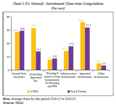 2.103 Surrenders and withdrawals have risen sharply, accounting for approximately 38.3 per cent of total pay-outs in 2025-26, going beyond maturity benefits which stood at 36.9 per cent. Death claims have normalised to around 8.1 per cent. The near parity between surrenders and maturity pay-outs indicates that policyholders are increasingly exiting policies prematurely. This shift has direct implications for asset-liability management (ALM), as early exits disrupt the long-duration assumptions underpinning life insurance investment strategies and can force asset liquidation ahead of schedule. Persistently elevated surrender rates also signal policyholder dissatisfaction, product mis-selling, or competitive pressure from alternative financial instruments. II.7.2.1.2 General Insurance Industry 2.104 Net incurred claims in the general insurance segment rose from ₹1.4 lakh crore in 2021-22 to ₹2.1 lakh crore in 2025-26, an increase of nearly 50 per cent over 5 years (Chart 2.54 a). This reflects rising frequency and severity of loss events, particularly in health and motor lines, which together constitute 95.3 per cent of net incurred claims in 2025-26 (Chart 2.54 b). 2.105 Health insurance claims have grown to 55 per cent of total net incurred claims, driven by medical inflation, rising hospitalisation rates and expanding coverage. Motor claims account for 40.3 per cent. The concentration of claims in these two segments creates correlated and structurally growing loss exposure that may strain reserving adequacy and underwriting margins, if not continuously recalibrated.
II.7.2.2 Expenses II.7.2.2.1 Life Insurance Industry 2.106 A distinct divergence in cost structure is evident between public and private life insurers. Private life insurers have seen commission ratio surge of almost 2 times from 2021-22, alongside a stable operating expense ratio (Chart 2.55 a and b). This escalation in distribution costs significantly outpaces private sector premium growth, compressing net margins and raising the risk of acquisition-cost-driven mis-selling. II.7.2.2.2 General Insurance Industry 2.107 In the general insurance segment, public insurers show a stable but elevated expense base. Operating expenses, after moderating in 2024-25, rose sharply again in 2025-26. Commission ratio has increased marginally for public insurers over the last 5 years (Chart 2.56 a). At the same time, private insurers’ commission expense ratio rose sharply, materially outpacing premium growth (Chart 2.56 b). This high cost of distribution for both public and private insurers act as a structural drag on underwriting margins, which are already negative across much of the sector.
II.7.2.3 Gross Yields II.7.2.3.1 Life Insurance Industry 2.108 The Life Fund of PSU insurer has shown an increasing trend, whereas the top nine private life insurers have exhibited a volatile trend over the 10-year period (Chart 2.57 a). The yields of the P&G Fund for both categories have exhibited a broadly declining trend over the period (Chart 2.57 b). This signals a structural reinvestment risk for annuity and pension obligations, a particularly sensitive issue as India’s ageing population increases, which need long-dated guaranteed liabilities in the sector. 2.109 ULIP Fund yields exhibit extreme volatility, consistent with the equity-heavy nature of ULIP investments (Chart 2.57 c). The high volatility of ULIP yields, while reflecting underlying policyholder risk, also highlights the mark-to-market sensitivity of this fund segment and its potential to generate near-term volatility in the insurance sector’s aggregate return metrics.  2.110 Par product yields have broadly tracked the Life Fund yield, which moved within a narrow 8.0-8.8 per cent band over 2021-22 to 2025-26. Non-Par products carry guaranteed return obligations, requiring insurers to earn at least the guaranteed rate from the fund. Two insurers have consistently outperformed, suggesting strong investment positioning. ULIP yields reflect total mark-to-market returns accruing to policyholders. Yields recorded a sharp dip in 2025-26, with the average sector fund yield at around 1.4 per cent, and only two insurers remaining above the average fund yield. Since policyholders bear investment risk under ULIPs, insurers’ balance sheets remain insulated, but sustained negative NAV performance materially elevates surrender risk. II.7.2.3.2 General Insurance Industry 2.111 The gross investment yields for the top 10 general insurers have trended broadly downward over the past decade, though shorter portfolio durations mean assets reprice faster than in the life segment, providing quicker benefit when rates rise (Chart 2.58). Investment income is critical to the profitability of general insurers, particularly where combined ratios remain elevated. Sustained yield compression, therefore, amplifies underwriting performance requirements, weighing on sector financial health. The trajectory of general insurers’ investment yields showcases an interplay between interest rate cycles, portfolio repositioning, and claims cost inflation, materially shaping the near-to-medium term financial outcomes. II.7.2.4 Equity Share Capital II.7.2.4.1 Life Insurance Industry 2.112 Life insurance sector’s equity capital grew from approximately ₹35,547 crore in 2021-22 to ₹42,627 crore in 2025-26 (Chart 2.59 a). The steady accumulation of core equity capital reflects the sector’s capacity to fund growth while maintaining solvency buffers. II.7.2.4.2 General Insurance Industry 2.113 General insurance sector’s equity capital has expanded more linearly and aggressively from approximately ₹37,855 crore in 2021-22 to over ₹44,824 crore in 2025-26(Chart 2.59 b). This continuous capital infusion reflects the structural necessity of absorbing persistent underwriting losses and supporting premium growth. While the sustained promoter support is a positive stability signal, the underlying drivers indicate that capital is being deployed defensively to plug recurring operating deficits rather than to support profitable expansion. II.7.2.5 Profitability II.7.2.5.1 Life Insurance Industry 2.114 A marked divergence in investment income patterns is observed between public and private sector insurers. Investment income remains the primary driver of life insurers’ profitability. PSU insurer’s investment income has grown steadily from approximately ₹2.9 lakh crore in 2021-22 to nearly ₹4.4 lakh crore in 2025-26, reflecting its large, sovereign-anchored asset base. Private insurers’ investment income, by contrast, has been significantly more volatile. 2.115 PSU insurer’s PAT rose to ₹57,419 crore in 2025-26. Private sector’s PAT has remained compressed at ₹7,576 crore in 2025-26, reflecting the persistent squeeze from high acquisition costs and earnings volatility. Total life sector’s PAT stands at around ₹65,000 crores in 2025-26 (Chart 2.60 a and b). II.7.2.5.2 General Insurance Industry 2.116 PSU underwriting losses widened in 2025-26. Standalone health insurers (SAHIs) and private insurers also recorded significant underwriting losses respectively for 2025-26 (Chart 2.61 a). Investment income continues to subsidise technical losses across the segment, with private insurers showing a stronger upward trend in investment earnings (Chart 2.61 b). However, this structural dependence on non-underwriting income as the primary profit stabiliser is a systemic vulnerability. Any compression in investment yields or capital market correction would directly erode the sector’s profitability buffer, exposing the inadequacy of underlying underwriting performance (Chart 2.61 c). II.7.2.6 Solvency II.7.2.6.1 Life Insurance Industry 2.117 The life insurance sector has remained solvency-compliant across all insurers through 2025-26, with no insurer falling below the regulatory minimum of 150 per cent (Table 2.16). However, the distribution of solvency ratios signals a notable downward trend within the compliant range. 2.118 A progressive migration of insurers from higher solvency bands toward the lower compliant range is observed. A large number of insurers operating with thin buffers above the minimum is structurally more vulnerable to simultaneous stress, particularly under adverse interest rate or equity market scenarios.
| Table 2.16: Life Insurance – Solvency | No. of Life Insurers with Solvency
(in per cent) | Q4: 2024-25 | Q1: 2025-26 | Q2: 2025-26 | Q3: 2025-26 | Q4: 2025-26 | | >225 | 9 | 10 | 7 | 6 | 3 | | >=200 to <225 | 5 | 3 | 6 | 8 | 2 | | >=175 to <200 | 8 | 10 | 9 | 9 | 15 | | >=150 to <175 | 3 | 2 | 3 | 2 | 5 | | <150 | 0 | 0 | 0 | 0 | 0 | Source: IRDAI
Note: Data for 2025-26 is provisional. | II.7.2.6.2 General Insurance Industry 2.119 The general insurance solvency picture is more mixed and structurally more concerning. Three insurers have remained below the 150 per cent regulatory minimum consistently across all five quarters from Q4:2024-25 to Q4:2025-26, a persistent non-compliance that represents a direct financial stability concern (Table 2.17). 2.120 The solvency ratio of general insurance segment shows greater quarterly volatility compared to the life segment. This volatility, combined with the structural presence of persistently sub-compliant entities and elevated underwriting losses, positions the general insurance sector as the more acute near-term concentration of capital risk in the broader insurance system. | Table 2.17: General Insurance – Solvency | No. of General Insurers with Solvency
(in per cent) | Q4: 2024-25 | Q1: 2025-26 | Q2: 2025-26 | Q3: 2025-26 | Q4: 2025-26 | | >225 | 10 | 11 | 11 | 11 | 10 | | >=200 to <225 | 6 | 7 | 8 | 8 | 3 | | >=175 to <200 | 8 | 8 | 7 | 4 | 10 | | >=150 to <175 | 7 | 5 | 5 | 8 | 8 | | <150 | 3 | 3 | 3 | 3 | 3 | Source: IRDAI
Note: Data for 2025-26 is provisional. | II.7.2.7 Grievance Analysis II.7.2.7.1 Life Insurance Industry 2.121 The life insurance sector shows a structural improvement in grievance experience. After peaking at over 1.5 lakh complaints in 2021-22, reported grievances declined to 1.2 lakh in 2025-26 (Chart 2.62 a). This improving trend suggests enhanced market conduct, better product suitability and more effective post-sale servicing. From a stability perspective, declining complaint volumes may reduce conduct-related reputational risk and support persistency improvements over time. II.7.2.7.2 General Insurance Industry 2.122 The general insurance sector presents a sharply contrasting picture. Reported grievances have nearly tripled to 1.78 lakh in 2025-26 (Chart 2.62 b). The steep and sustained rise in grievances indicates systemic shortfalls in claims management, service quality and product communication. Unresolved conduct risk of this scale can erode policyholder trust, reduce renewal rates and ultimately become a financial stability concern if it precipitates mass policy exits. II.7.3 Scenario Analysis II.7.3.1 Policyholders’ Funds vs. Shareholders’ Funds 2.123 The solvency margin, which is defined as the excess of available solvency margin (ASM) over required solvency margin (RSM), is the primary measure of insurer financial resilience. The ASM of insurers is bifurcated between ‘excess in policyholders’ funds’ and ‘excess in shareholders’ funds’, providing a granular view of where solvency buffers exist. II.7.3.1.1 Life Insurance Industry 2.124 The shareholders’ fund component of the PSU insurer’s ASM has progressively increased from 2022-23, aligning it with broader industry practice (Chart 2.63 a). For the top nine private insurers, ASM composition remains stable, with shareholders’ funds accounting for a structurally higher share, reflecting their greater proportion of non-participating and unit-linked business (Chart 2.63 b). II.7.3.1.2 General Insurance Industry 2.125 For the four General PSUs, the ‘excess in policyholders’ funds’ has contributed negatively to the ASM for 2024-25 and 2025-26 (Chart 2.64 a). For the top 6 private General insurers, the ASM composition is stable (Chart 2.64 b). The negative contribution of policyholders’ funds to the ASM of the 4 General PSUs is a financial stability signal. This structural weakness leaves the ASM of public sector general insurers increasingly dependent on shareholder capital infusions and investment income, both of which are subject to external factors. If this trend persists, the capital adequacy of PSU general insurers will become progressively more sensitive to government capital support decisions, an important contingent fiscal risk.
II.7.3.2 Scenario Analysis – Resilience of Solvency Margin 2.126 To assess the resilience of life and general insurers’ solvency positions under adverse conditions, the above five stress scenarios were constructed, combining simultaneous shocks to the ASM and the RSM. These scenarios range from mild to severe stress: direct erosion of the capital buffer, a disproportionate squeeze on ASM relative to RSM and a surge in RSM driven by elevated risk exposures. The regulatory solvency ratio threshold of 1.5 times the RSM serves as the benchmark for evaluating insurer resilience across scenarios. These stress scenarios, while constructed as abstract shocks to the ASM and RSM, are grounded in the macroeconomic transmission channels described above. The mild (S1) and moderate (S2) scenarios are consistent with short-cycle disruptions, such as transient interest rate volatility or a moderate equity market correction, where mathematical reserves face limited revaluation pressure and investment portfolio losses remain contained. The severe scenario (S3) broadly reflects conditions associated with a significant macroeconomic downturn or a sharp but recoverable market dislocation, wherein deteriorating asset quality, rising claims provisions and elevated reinvestment risk simultaneously pressure both sides of the solvency equation. The margin squeeze scenario (S4) is most representative of an environment in which geopolitical shocks trigger mark-to-market losses on fixed-income and equity portfolios, compressing admissible assets faster than required margins can be adjusted. The RSM spike scenario (S5) mirrors conditions of regulatory reserve strengthening (Table 2.18). | Table 2.18: Shock Scenarios | | (per cent) | | Scenario | ASM Shock | RSM Shock | Description | | S1 Mild | -5.00 | +5.00 | Mild direct solvency stress | | S2 Moderate | -10.00 | +10.00 | Moderate direct solvency stress | | S3 Severe | -15.00 | +15.00 | Severe direct solvency stress | | S4 Margin Squeeze | -20.00 | +10.00 | ASM falls faster than RSM rises | | S5 RSM Spike | -10.00 | +20.00 | Required margin shock dominates | | Source: IRDAI. | II.7.3.2.1 Life Insurance Industry 2.127 The results of scenario analysis of top 10 life insurers reveal a progressive deterioration in sector-wide solvency compliance as stress intensity increases (Chart 2.65 a and b). Under the mildest scenario (S1), all 10 insurers continue to maintain solvency ratios above the 1.5x threshold, suggesting that most insurers hold capital buffers comfortably in excess of regulatory requirements under mild stress (Table 2.19). However, as the severity of the shock escalates, compliance narrows sharply, declining to 8 insurers under the moderate scenario (S2), and falling further to only 4 insurers each under the severe (S3) and margin squeeze (S4) scenarios. The RSM spike scenario (S5) results in only 4 insurers remaining above the threshold. 2.128 These findings underscore a bifurcation in the sector’s solvency landscape. While the majority of insurers are adequately capitalised to absorb mild-to-moderate stress, a subset of entities exhibits limited buffers above the regulatory floor, rendering them vulnerable to more severe dislocations (Chart 2.65 c). The concentration of stress impact in the lower tail of the solvency distribution warrants close supervisory attention, particularly as market volatility, claims experience and interest rate movements can simultaneously compress ASM and elevate RSM, replicating conditions broadly consistent with the S4 or S5 scenarios. | Table 2.19: Life Insurer-wise Distribution of Solvency | | Scenario | Number of Insurers above 1.5x | | S1 Mild | 10 | | S2 Moderate | 8 | | S3 Severe | 4 | | S4 Margin Squeeze | 4 | | S5 RSM Spike | 4 | | Source: IRDAI. | II.7.3.2.2 General Insurance Industry 2.129 The results of the scenario analysis for the top 10 general insurers reveal that the sector exhibits a tighter capital buffer relative to the life insurance segment, with a smaller number of insurers maintaining compliance above the 1.5x threshold at each level of stress (Chart 2.66 a). Under the mild scenario (S1), 7 of the top 10 general insurers remain above the regulatory threshold, indicating that while the majority of the sector is adequately capitalised under moderate stress, a meaningful proportion operates with limited headroom even under mild adverse conditions (Chart 2.66 b). As stress intensity escalates, compliance narrows progressively, declining to 6 insurers under the moderate scenario (S2) and to 4 under the severe scenario (S3) (Table 2.20). The margin squeeze scenario (S4), results in only 3 insurers maintaining the threshold, underscoring the particular vulnerability of capital-thin general insurance entities to scenarios where underwriting losses and reserve strengthening simultaneously erode the available margin. The RSM spike scenario (S5), with 5 compliant insurers, highlights that a surge in required capital, driven by elevated risk exposures, can be as destabilising as a direct erosion of the solvency buffer. 
| Table 2.20: General Insurer-wise Distribution of Solvency | | Scenario | Number of Insurers above 1.5x | | S1 Mild | 7 | | S2 Moderate | 6 | | S3 Severe | 4 | | S4 Margin Squeeze | 3 | | S5 RSM Spike | 5 | | Source: IRDAI. | 2.130 Taken together, these findings point to a sector-level solvency distribution in which a subset of general insurers, particularly those with elevated combined ratios or concentrated underwriting exposures are meaningfully exposed to regulatory breach under stress conditions more severe than S2 (Chart 2.66 c). The general insurance industry’s relatively shorter asset-liability duration and greater sensitivity to annual underwriting outcomes amplify the speed with which adverse developments can translate into solvency deterioration, reinforcing the need for proactive capital management and continuous supervisory engagement with entities operating close to the regulatory minimum. 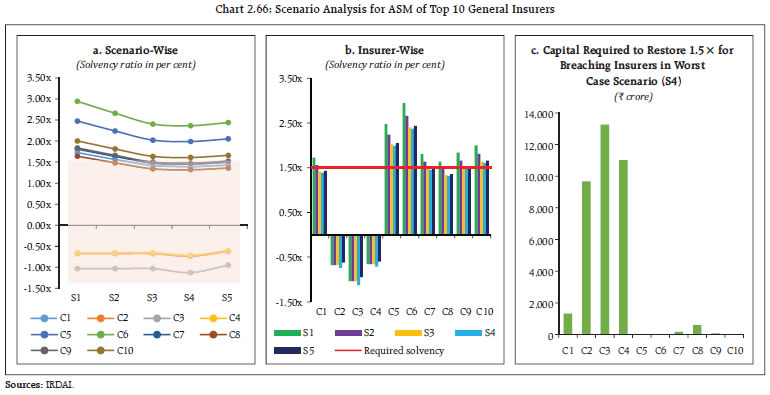 . II.7.3.3 Capital Buffer above Regulatory Minimum Solvency II.7.3.3.1 Top 10 Life Insurers 2.131 The capital buffer above the regulatory minimum solvency measures the excess capital headroom that insurers maintain over and above the 1.5 times Required Solvency Margin (RSM) threshold. This metric provides a forward-looking lens on sector resilience, capturing not merely whether an insurer is compliant, but the degree of additional shock it can absorb before breaching the regulatory floor. 2.132 For the PSU insurer, the capital buffer is of more than rupees one lakh crore for 1.5x solvency and more than rupees fifty thousand crore for 2.0x solvency. For top 9 private life insurers, the analysis of the buffer distribution reveals a polarised capital landscape. A majority of insurers maintain solvency ratios significantly in excess of the 1.5x threshold. However, for 2.0x solvency, a cohort of insurers operates with relatively thin buffers, leaving them with limited cushion to absorb unexpected shocks (Chart 2.67). II.7.3.3.2 Top 10 General Insurers 2.133 The capital buffer above the regulatory minimum solvency for the top 10 general insurers captures the excess of each insurer’s actual solvency ratio above the mandatory 1.5x RSM threshold. In contrast to the life insurance sector, where the solvency buffer tends to be structurally more stable due to the long-duration and predictable nature of life liabilities, the solvency buffer in general insurance is subject to greater annual volatility, driven by the sensitivity of claims outcomes to catastrophic events, adverse loss development and underwriting cycle fluctuations. Accordingly, maintaining an adequate buffer above the regulatory minimum is especially critical in the general context (Chart 2.68). 2.134 An analysis of the capital buffer distribution across the top 10 general insurers reveals a heterogeneous picture. Several well-capitalised private general insurers maintain solvency ratios significantly above the 1.5x threshold. However, a cluster of insurers operates with narrower capital cushions. 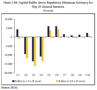 2.135 The heterogeneous capital buffer distribution in the general sector, with a cluster of insurers operating with narrow cushions, represents the most acute near-term financial stability concern in the insurance sector. Unlike in the life sector, where long-duration liabilities allow gradual capital rebuilding, general solvency buffers can be depleted rapidly in a single adverse underwriting year, as natural catastrophes, pandemic events, or judicial award spikes demonstrate. The combination of thin buffers, elevated combined ratios and declining investment yields in a subset of general entities creates a scenario where a moderate macro-financial shock could trigger simultaneous multi-insurer solvency stress, with potential spillovers. Robust capital planning, including pre-emptive capital raising by at-risk entities, is the primary mitigation. II.7.4 Emerging Areas of Stress in Insurance Sector 2.136 While the insurance sector remains broadly resilient, several underlying structural pressures exist from a financial stability perspective. Sustained premium expansion has strengthened the sector’s ability to absorb shocks. However, elevated surrender behaviour in life insurance points to weaker policy persistency and introduces uncertainty in asset-liability management. In general insurance, rising claims intensity and concentration of claims in health and motor segments have increased pressure on underwriting performance, reinforcing dependence on investment income as a stabilising source of profitability. Further, increasing distribution costs, particularly in private life and general insurance segment, continue to affect policyholder value and compress margins. Moreover, rising policyholder grievances in general insurance segment indicates gaps in service quality. 2.137 A gradual movement of insurers towards thinner solvency cushions, along with continued dependence on capital infusion by 3 public sector general insurers, highlight the need for stronger capital resilience. At the same time, heavy concentration of investment portfolios in sovereign securities exposes insurers to interest rate volatility and limits portfolio flexibility. Further, prolonged yield compression may intensify reinvestment challenges, especially for long-duration liabilities in life insurance. 2.138 Addressing these pressures through improved underwriting discipline, stronger capital buffers, better alignment of distribution incentives with persistency, and enhanced customer outcomes would be essential for reinforcing the sector’s long-term resilience and sustaining broad-based insurance development, supported by structural and operational reforms as envisaged in the Sabka Bima Sabki Raksha (Amendment of Insurance Laws) Act, 2025. 2.139 Beyond these traditional pressures, emerging risks such as climate change, cyber threats and geopolitical uncertainty are adding new dimensions to the sector’s risk profile. 2.140 Taken together, these risks highlight that the sector’s vulnerabilities are no longer confined to underwriting performance alone but also stem from climate, technology, market, geopolitical and operational risks.
|