Press Release RBI Working Paper Series No. 01 Data Gaps in State-Level Inflation: An Assessment for the Covid Period Purnima Shaw and R. K. Sinha@ Abstract 1 The disruption during Covid-19 necessitated statistical organisations across the world to impute the missing official statistics data or explore alternative data sources. The Reserve Bank of India’s (RBI’s) Inflation Expectations Survey of Households (IESH) continued to be conducted (using telephonic interviews) during the pandemic months. While imputed figures for the official price indices are available at the aggregate level for April and May 2020, the State-wise inflation data remains unpublished (missing) for four of the pandemic months. This paper uses granular IESH data and takes a distributional approach to provide State-wise inflation estimates for these data gaps. These State-wise inflation estimates when aggregated, closely follow the all-India official CPI inflation series. JEL Classification: D84, E17, E31 Keywords: Consumer price index, distribution function, inflation, inflation expectations Introduction The outbreak of the coronavirus (Covid-19) pandemic across the globe and the related administrative measures implemented to control its spread, e.g., closure of non-essential businesses, public offices and restricted movements resulted in a severe disturbance in the routine compilation and dissemination of official statistics. In such a scenario, the compilers of official statistics, like Central Banks and National Statistical Offices across the world needed to retain the confidence of the users of official statistics in the data. The need of the hour was to ensure complete transparency in the data collection and dissemination processes. A possible way forward was to make concerted efforts to collect the required data, drawing on both current and alternative sources, to compile reliable statistics and cover data gaps using universally accepted methodologies. Statisticians in various data compiling positions, were proactive in handling these challenges and exploring new ways to address the gaps in collection of data. The challenges in the compilation of the Consumer Price Indices (CPI) were profound. During the Covid period of restricted movement, limited shops were operational, and several consumer items were unavailable in shops because of supply chain issues. In addition, restrictions on physical movement made data collection for the limited available items largely unfeasible. Further, the ability to conduct surveys was also impacted severely. Statisticians around the world had to adapt to these data compilation challenges and adopt various methodologies available in the literature for addressing missing data. To fill-in the missing information, data imputation was followed mostly across the economies. In spite of these, several challenges were being faced by the data users including Central Banks across the world in analysing these imputed official statistics which included uncertainty in the imputed figures; changes in the consumption basket due to pandemic related supply constraints resulting in biased price deflators; delay in data dissemination; frequent revisions in data and its composition; changes in data collection methodology; varying seasonal patterns in data; uncertainty in data biases (e.g., time variation, impact of the changing economy and policy actions); sample representativeness due to limited access; outdated profile of survey respondents; changes in time series trends leading to the risk of increasing bias in estimates; reduced response rates with less accurate responses due to pandemic-related priorities; and constraints related to auxiliary data sharing because of limited resources and delays due to the pandemic (Beer and Tissot, 2021). To address the need for analysing timely data during the pandemic induced uncertainties, Central Banks required high frequency data from alternative sources in place of the traditional sources (Hinge, 2020). High frequency data sources were used to decipher the dynamics of important macroeconomic conditions. The use of such high frequency data in this regard were proved to be useful in studies by Hopkins and Sherman (2020) for Ireland, Bank of Japan (2020), Davies et al. (2020) for Bank of England and Chapman and Desai (2021) for Canada. However, these high frequency data have their own limitations as they need to be adjusted for seasonality, weather conditions, and other relevant factors (Castelletti et al., 2020 and Beer and Tissot, 2021). Further, innovative methods needed to be quickly explored for dealing with the methodological issues induced by the range of vast policy measures being taken by administrative authorities in response to the pandemic. Beer and Tissot (2021) suggested better use of existing big data sources, taking advantage of the progressing digital innovation for building automated link within granular datasets. In spite of all these efforts, certain gaps remain in official statistics during the pandemic period, resulting in a break in the time series data. While data on several commodity prices were imputed across economies, including India, there remain certain data gaps during the pandemic period, due to insufficient data collection. In case of India, imputed price indices for the official inflation were released at the aggregate level for the months of April and May 2020. However, the State-wise official inflation figures are missing for four of the pandemic months. Taking cues from Shaw and Sinha (2024) which highlights the importance of the granular dataset on the RBI’s IESH in nowcasting and forecasting State-wise inflation figures, and adaptive nature of the households’ inflation expectations in India, the current paper makes a novel attempt of using households’ inflation perceptions and expectations to present urban inflation estimates for the States for the pandemic months of April and May, 2020 and 2021. Section II of the paper reviews various data imputation techniques from the existing literature followed by cross country estimates and use of alternative data for imputation. Section III explains the proposed methodology for estimating the missing State-wise urban inflation data. The first part of Section IV examines the performance of the proposed methodology using existing data and then proposes State-wise estimates for the months of April and May 2020 and 2021. This is followed by the concluding remarks in Section V. II. Estimation of Missing Time-Series Data Missing data may arise due to a random mechanism or a structural deficiency. The structural deficiency indicates that a component of data is omitted. Random missing mechanism can be classified into three categories as follows (Kuhn and Johnson, 2020): i. Missing Completely at Random (MCAR): The missing data is due to a random mechanism and the probability of missingness is same for the existing as well as missing data. An example of this could be missing price data due to the closure of a shop with significant business profile. ii. Missing at Random (MAR): The probability of missingness is not the same for the existing and missing data and it depends on the existing data and not on the missing data. Observed data can be used to predict the missing data. For example, missing data on quarterly gross domestic product (GDP) of a financial year can be approximated with the help of available annual GDP estimate and past quarterly GDP estimates. iii. Not Missing at Random (NMAR): The missing data is related to the non-observed data. The missingness is due to the factors which are not considered during data collection. For example, data on sensitive economic variables like individual income, savings, etc. The missing CPI data during Covid period can be classified as Missing Completely at Random (MCAR). If the missing mechanism is MCAR and the loss is low, then ignoring/ deleting the missing data can be a feasible option (Ribeiro and Castro, 2022). However, the loss in this case is significant and cannot be afforded, as deletion will result in a break in time series, thereby impacting the entire forecasting process and analysis. Hence, data imputation becomes necessary for estimating the missing CPI data for the pandemic period. A few imputation techniques following Pratama et al. (2016), Ribeiro and Castro (2022) and Rocha et al. (2024), are mean, median and mode imputation which replace the missing data with mean, median or mode of the remaining features (other related variables) of the data. This is suitable for stationary time series data; hot deck imputation which searches for data on features like those related to the sample on missing data and replace the missing data with a random data from the similar sets (Andridge and Little, 2010); cold deck imputation which replaces the missing data with a random data from the similar sets from a different data source (Duma et al., 2013); forward and backward filling which replaces missing data with the last observed data (forward filling) or with the next observed data (backward filling) under the assumption that missing data is similar to the adjacent data points (Molnar et al., 2008). However, this method creates an issue if there is seasonality in the variable. Other techniques include multiple imputation which calculates multiple imputed values with a probability distribution for a missing data. These data are examined and combined to generate realistic estimate (Azur et al., 2011). The method is suitable for imputing missing data in survey with MAR mechanism. Linear interpolation techniques have been used to compute using a linear function to connect the nearest points to represent the data well while spline interpolation has been used for computing missing values using a polynomial function to connect the nearest points to represent the data well (Elissavet, 2017). Holt’s (1957) exponential weighted moving average can also be used wherein, the imputed figure is derived as a weighted average of the historical data points. The weighting factors reduce exponentially for the older time points. Fix and Hodges’ (1951) k-nearest neighbour method is appropriate when the distribution of the data is unknown. The method uses the average or median of the target values from the k nearest neighbours to make a prediction of the missing value. Kalman prediction (pioneered by Swerling, 1958, Kalman, 1960 and Kalman and Bucy, 1961) is a linear model of estimation based on an algorithm and consists of two processes: a prediction stage and a correction stage. In missing indicators method, for each of the partially observed feature, a corresponding indicator variable is added to indicate the missingness using binary values. It can be used with any imputation method, but is most commonly used with mean imputation (Groenwold et al., 2012). Expectation maximisation method uses other features to impute the missing value and then checks whether it is the most probable value. This step is iterated till the most probable value is found (Dempster et al., 1977). Other recent imputation methods include ST-2SMR (Cheng and Lu, 2017), temporal belief memory (Kim and Chi, 2018), long short-term memory (Patterson and Gibson, 2017) and generative adversarial imputation network (Yoon et al., 2018). II.1. Cross Country Experiences Cross-country experiences show a wide-range of techniques that were used by various economies to fill-up the gap in commodity prices during Covid-19 period. The Office for National Statistics in the U.K. imputed2 the prices of items which were either unavailable or available in a limited manner. The imputation was based on the method that best reflected the price behaviour of the missing commodity. The imputations were based on three methods: first, using the price index immediately above the item in classification structure; second, using the price movement of a similar commodity; and third, applying forward filling. For imputing a missing price of non-seasonal commodities, combined monthly growth of all available non-imputed commodity prices was used. The U.S. Bureau of Labor Statistics imputed missing prices using cell-relative imputation method3. In this method, imputed price is derived using the average price change of all items similar to the missing item in one month for the same geographic area. This method is used for commodities where it may be safely assumed that the price changes in the missing items would be similar to the price changes in the other items. The U.S. Bureau of Labor Statistics listed down items for which data was inadequate for publication during each of the pandemic months. The Australian Bureau of Statistics used three types of imputation4 techniques. For available goods and services, for which prices were temporarily unavailable, imputed price was taken as the average price change of similar goods and services. For unavailable goods and services, where a significant amount of its typical expenditure has been substituted to another good or service, donor imputation technique was used, wherein price change of a donor commodity is considered. For unavailable goods and services, where expenditure cannot be substituted by any other commodity, prices were imputed off the headline CPI. The Department: Statistics South Africa (Stats SA) practiced two types of imputation techniques5. The price change of commodities for which no expenditure was possible due to the restricted movement, imputed prices were taken as the change in the headline CPI index of all items based on those products, for which prices were either available or imputed by other methods. For the items which are either quarterly or annually collected, the previous month’s corresponding indices were carried forward. The price change in diesel was imputed using the change in the regulated wholesale price of diesel. Certain items under the personal care group were possibly available for sale, but their prices could not be collected, and therefore, were imputed by the personal care index. In India, the Ministry of Statistics and Programme Implementation (MOSPI) imputed6 the prices of sub-groups under the food group by multiplying the last observed index of the sub-group with the price relative of food group index calculated based on the available prices. Imputation of the prices of sub-groups under the non-food group were done by multiplying the last observed index of the sub-group with the price relative of general CPI index calculated based on the available prices. | Table 1: Data Gap in CPI in India | | Month | Area | | Index | | | Inflation | | Rural | Urban | Combined | Rural | Urban | Combined | | March 2020 | 36 States | ✓* | ✓* | ✓* | ✓* | ✓* | ✓* | | India | ✓ | ✓ | ✓ | ✓ | ✓ | ✓ | | Items | NA | NA | | NA | NA | | | April 2020 | 36 States | | | | | | | | India | ✓# | ✓# | ✓# | ✓# | ✓# | ✓# | | Items | NA | NA | | NA | NA | | | May 2020 | 36 States | | | | | | | | India | ✓# | ✓# | ✓# | ✓# | ✓# | ✓# | | Items | NA | NA | | NA | NA | | | March 2021 | 36 States | ✓* | ✓* | ✓* | ✓* | ✓* | ✓* | | India | ✓ | ✓ | ✓ | ✓ | ✓ | ✓ | | Items | NA | NA | ✓ | NA | NA | | | April 2021 | 36 States | ✓* | ✓* | ✓* | | | | | India | ✓ | ✓ | ✓ | ✓ | ✓ | ✓ | | Items | NA | NA | ✓ | NA | NA | | | May 2021 | 36 States | ✓* | ✓* | ✓* | | | | | India | ✓ | ✓ | ✓ | ✓ | ✓ | ✓ | | Items | NA | NA | ✓ | NA | NA | | ✓ Available.
✓ # Imputed figure is available.
* For Arunachal Pradesh, only rural indices and inflation are available for both pre- and post-Covid periods. | | ‘NA’ – Combined figures for CPI indices and inflation are released by MOSPI; rural and urban classifications are not published. | | Source: MOSPI. | Despite extensive use of imputation techniques in presenting missing CPI values during the pandemic period, there exists missing data in the CPI in India. During the months of April and May 2020, the complete CPI State-wise data could not be collected due to the restrictions imposed to curb the spread of Covid-19. The MOSPI released the CPI provisional indices for select groups and sub-groups for the months of April and May 2020 on the 12th day of May and June, 20207 respectively. These releases stated that the general indices and State-wise indices could not be compiled. Later, on July 13, 2020, a technical note8 was released which contained imputed general indices for both the months. However, the State-wise estimates could not be constructed as the number of price quotations received (through both telephonic conversations and physical visits to neighbourhood shops) was insufficient. In the year 2021, State-wise indices were released for both the months of April and May, but the inflation could not be compiled due to the absence of the indices in the corresponding months in 2020. As a result, there remains a break in the State-wise inflation series for the months of April and May during the years 2020 and 2021. The blank cells in Table 1 show the existing gaps in the CPI data. The cells highlighted in green represent the gaps, which this paper attempts to fill-in. II.2. Use of Alternative Data Sources for Imputation Apart from the above-mentioned methodologies on imputation, there have been attempts of estimating the missing data by making use of alternative data sources. Cavallo (2020) used the credit and debit card transactions between the first five months of 2020 and presented inflation estimates for the U.S. economy. These were found to be higher than the official inflation. The gap ranges from 0.1 percentage points in March 2020 to 0.7 percentage points in April 2020 followed by 0.8 in May 2020. Based on bank card transactions, Gautier et al. (2023) calculated similar estimates for France from January to December 2020. Their estimates were also on the higher side with the largest gap being 1.1 percentage points in April 2020. Using debit card data, Jonckheere and Zimmer (2020) presented such revised estimates for Belgium from February to July 2020. The estimates were on the higher side than the official inflation from March 2020 to July 2020. Kouvavas et al. (2020) used aggregate turnover data to estimate the changing consumption patterns and derived revised inflation figures for the Euro area from January to August 2020. With a finding similar to the above-mentioned ones, the gap between the estimates and the official inflation peaked to 0.25 percentage points in May 2020. The findings of Huynh et al. (2020) indicate marginal uptick in the estimated inflation obtained using high frequency expenditure network data (on debit card purchases) from the official inflation during March, April and May 2020 in Canada. The differences are 0.1, 0.2 and 0.3 percentage points, respectively. Taking cue from these literatures which have used alternative data sources to estimate the inflation of the missing data during the Covid period, this paper attempts to make use of an alternative dataset in case of India, i.e., the RBI’s IESH granular data to derive estimates for the missing data in the State-wise CPI inflation. A recent study by Shaw and Sinha (2024) used the granular IESH data to nowcast and forecast the State-wise inflation figures. The current paper makes a novel attempt of using this data to present urban inflation estimates for the States for the pandemic months of April and May, 2020 and 2021, for which the CPI inflation data are missing. III. Methodology The use of alternative data sources in computing estimates of the unobservable economic variables during the pandemic period has been discussed in Section II. Alternative data may provide only limited information during normal periods of the economic cycle. However, such data are more indicative of the situation during crisis periods, more so for the short term (INSEE, 2020). RBI’s IESH data related to inflationary sentiments may be considered as an alternative dataset and hence, it has been used extensively in this paper9. The RBI’s Survey of Professional Forecasters (SPF) is also a rich dataset on all-India inflation forecasts; it cannot be used to study State-wise inflation estimates. This paper attempts to fill-in the missing data on State-wise inflation for April and May, 2020 and 2021. State-wise inflation data are particularly important for studying State-specific information like inter-State transportation costs, State taxes, differences in States for supply chain management, etc., all of which contribute to the inflation volatility amongst States. The centre-wise survey data are also important for the study as various factors like respondents’ age, gender, occupation, location, etc., impact the sentiments of survey respondents rendering variability in the sentiments among various centres. Accordingly, the availability of estimates for the State-wise inflation for the specific months, which remains unpublished, would be potentially useful for any relevant study involving State-level inflation time-series data going forward, as the proposed estimates attempt to resolve the break in State-wise inflation series, to an extent. During the Covid-19 pandemic and amid the ensuing restrictions, IESH managed a full-sample response by switching to either fully telephonic or a combination of telephonic and physical interviews during the rounds of May 202010, July 202011, September 202012, November 202013, January 202114, May 202115, July 202116 and September 202117. Taking cue from the adaptive nature of the households’ inflation expectations in India (Sharma and Bicchal, 2018, Shaw, 2019, Singh et al., 2024, Shaw, 2024, to name a few), RBI’s IESH18 may be considered as an alternative data to make a plausible conjecture about the State-wise inflation dynamics during April and May, 2020 and 2021, when inflation was volatile due to the disturbances in the demand-supply dynamics. Recently, Shaw and Sinha (2024) attempted a novel method of mapping distributions of the centre-wise granular IESH data from the survey to the State-wise granular CPI-urban (CPI-U) inflation data to present State-level CPI-U inflation nowcasts and forecasts. Further, it is reasonable to expect that the demand-supply shocks due to the unprecedented pandemic must have impacted the CPI inflation as well as the households’ sentiments (Chart 1), making the latter even more relevant to use for the purpose. This section proposes a methodology for arriving at the inflation estimates of the urban19 areas of the States in which IESH is conducted for the months of April and May for the years 2020 and 2021. The exercise will be able to present urban inflation estimates for select States in the highlighted cells in Table 1. 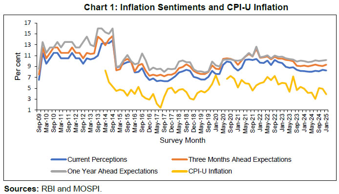 The responses on inflation perceptions and expectations are collected in buckets of (<1%,1−<2%,…,15−<16%,≥16%). The respondents with inflation perception/ expectation beyond 15 per cent are requested to provide the exact inflation number. General characteristics of the data include the respondents’ preferences in polling their inflation perceptions and inflation expectations in multiples of five (Chart 2) (Sinha, 2023 and Shaw and Sinha, 2024). This makes the data distribution uneven and adds to the variation across the survey centres. Looking at the sample frequency distribution of inflation perceptions/ expectations of each of the survey centres for each of the study periods, the distribution can be smoothened by removing the sudden frequency spikes due to digit preference and by replacing such frequencies with approximate values obtained using interpolation method20. Here, the frequencies at multiples of 5 are assumed to be unknown and interpolated using the nearby frequencies. Let fi be the frequency for the ith response class. Let x be a continuous variable indicating responses and f(x) be a function of x representing the corresponding frequencies. Consider n values of f(x) are known and assume that f(x) is a polynomial of (n − 1) degrees,  respectively. Thus, the frequencies at multiples of 5 are replaced with positive interpolated frequencies, which make the sample frequency distribution smoother than the previous one. The properties (moments) of the smoothed distribution will not be like the true frequency distribution (captured in the survey) because the peaked frequencies at multiples of 5 observed due to respondents’ digit preference are averaged out. It appears that by doing so, there is information loss, but this is undertaken so that a workable and standard probability distribution can be fitted to the survey data. Shaw and Sinha (2024) have used the residual data (peaked frequencies) to nowcast and forecast the CPI inflation. These modified sample distributions are then fitted with various continuous probability distributions, viz., Normal, Laplace, Log-normal, Gamma, Logistic, Weibull and Log-logistic distributions and among these, an appropriate distribution is selected for fitting using the non-parametric Kolmogorov-Smirnov’s test for goodness of fit. Let g(x) be the fitted distribution. Considering the distribution of the official CPI-U inflation (of eight months21 previous to the survey month) of each of the 17 States, where IESH is conducted for each of the 47 survey rounds, there are 799 distributions. These sample distributions are also fitted with the aforementioned seven probability distributions and an appropriate distribution is selected and fitted using the Kolmogorov-Smirnov’s test. Let h(y) be the fitted distribution and F(y) be the cumulative distribution function such that, for any real number “a”, Corresponding to the probabilities g(x), the percentiles of F(a) can be tabulated using, Using this derived distribution, the modal value from the distribution is taken as the inflation nowcast/ forecast. The nowcasts/ forecasts, thus derived, may be considered as the inflation estimates for the months for which CPI-U inflation data is missing. IV. Numerical Illustration Before moving on to fill-in the State-wise inflation data gap, it is necessary to apply the estimation techniques to the periods, for which the official inflation data are available. This will facilitate in gauging the quantum of error in the estimates using the methodology described in the previous section. For this purpose, centre-wise inflation perceptions and three-months ahead inflation expectations are considered from the IESH data for the 47 survey rounds during September 2016 to May 2024. One year ahead inflation expectations of consumers are not considered with the logic that such expectations would likely reflect outdated information in a rapidly evolving economic environment. The objective is to first examine the performance of inflation nowcasts using consumers’ inflation perceptions. Thereafter, the performance of three-months inflation forecasts, which were computed using consumers’ three-months ahead inflation expectations are to be testified. Given a survey centre for each of the 47 survey rounds above, corresponding State’s official CPI-U data for the previous eight months are taken as the reference data. For example, if it is required to nowcast CPI-U inflation of Gujarat for May 2024, then the survey data of Ahmedabad for the round May 2024 and CPI-U inflation data of Gujarat for the months September 2023 to April 2024 are considered. Further, for three months ahead forecast, in order to forecast the CPI-U inflation of Gujarat for April 2024, the survey data of Ahmedabad for the survey round January 2024 and CPI-U inflation data of Gujarat for the months May 2023 to December 2023 are considered. There are 18 urban survey centres in the IESH data22, which are assumed to represent the urban areas of the respective 17 CPI States23. Considering the sample distribution of inflation perceptions/ expectations of each of the 18 survey centres for each of the 47 survey rounds, there are 846 distributions. A city-wise distribution of the responses (including exact responses beyond 15 per cent) for the study period in Chart 2 reflects the concentration of responses in multiples of 5, indicating the digit preference of respondents in polling inflation perceptions/ expectations. The intensity is, however, dying out with the increase in numbers. The responses are henceforth considered up to 20 per cent, representing about 92 per cent (89 per cent) of the inflation perceptions (three months ahead inflation expectations). The interpolated frequencies are obtained for frequencies at 5−<6%, 10−<11%, 15−<16% and 20% using equations 7 to 22. 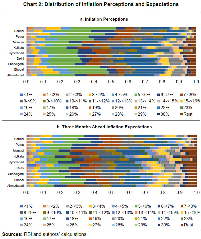 Following the methodology described in Section III, the nowcasts and three months ahead inflation forecasts are obtained, and their performances with respect to the official CPI-U inflation figures (published by MOSPI), are gauged using the standard measures defined below: where, FEt = Ft - At
Ft = forecast for time periodt
At = actual at time periodt
T = number of time periods The nowcasts and forecasts are also consolidated for all the survey States using weighted average, where CPI-U State weights are used. For Maharashtra, the nowcasts/ forecasts of Mumbai and Nagpur are averaged. The State-wise errors given in Table 2 below, show that the nowcast/ forecast errors of the States, viz., Karnataka, Maharashtra and Kerala, are relatively lower than those of the other States. | Table 2: Forecast Errors | | Nowcasts for September 2016 to May 2024 | RMSE | | Gujarat | 1.454 | Delhi | 1.241 | Uttar Pradesh | 1.672 | Jharkhand | 1.485 | | Karnataka | 1.088 | Assam | 1.581 | Maharashtra | 1.079 | Chhattisgarh | 1.852 | | Madhya Pradesh | 1.333 | Telangana | 1.864 | Bihar | 2.006 | | | | Odisha | 1.662 | Rajasthan | 1.486 | Kerala | 1.057 | | | | Tamil Nadu | 1.468 | West Bengal | 1.957 | Chandigarh | 1.635 | | | | Survey States Combined* - 1.073 | | MAE | | Gujarat | 1.181 | Delhi | 0.973 | Uttar Pradesh | 1.302 | Jharkhand | 1.233 | | Karnataka | 0.835 | Assam | 1.233 | Maharashtra | 0.878 | Chhattisgarh | 1.435 | | Madhya Pradesh | 1.120 | Telangana | 1.345 | Bihar | 1.644 | | | | Odisha | 1.281 | Rajasthan | 1.190 | Kerala | 0.823 | | | | Tamil Nadu | 1.251 | West Bengal | 1.576 | Chandigarh | 1.219 | | | | Survey States Combined* - 0.849 | | MAPE | | Gujarat | 0.345 | Delhi | 0.311 | Uttar Pradesh | 0.367 | Jharkhand | 0.298 | | Karnataka | 0.205 | Assam | 0.286 | Maharashtra | 0.205 | Chhattisgarh | 0.550 | | Madhya Pradesh | 0.274 | Telangana | 0.439 | Bihar | 1.210 | | | | Odisha | 0.329 | Rajasthan | 0.285 | Kerala | 0.180 | | | | Tamil Nadu | 0.301 | West Bengal | 0.371 | Chandigarh | 0.760 | | | | Survey States Combined* - 0.213 | | Three Months Ahead Forecasts for December 2016 to August 2024 | RMSE | | Gujarat | 1.547 | Delhi | 1.572 | Uttar Pradesh | 1.993 | Jharkhand | 1.506 | | Karnataka | 1.292 | Assam | 2.201 | Maharashtra | 1.386 | Chhattisgarh | 2.272 | | Madhya Pradesh | 1.474 | Telangana | 2.064 | Bihar | 2.113 | | | | Odisha | 1.860 | Rajasthan | 1.662 | Kerala | 1.046 | | | | Tamil Nadu | 1.678 | West Bengal | 2.893 | Chandigarh | 1.617 | | | | Survey States Combined* - 1.178 | | MAE | | Gujarat | 1.229 | Delhi | 1.242 | Uttar Pradesh | 1.558 | Jharkhand | 1.310 | | Karnataka | 1.040 | Assam | 1.835 | Maharashtra | 1.141 | Chhattisgarh | 1.816 | | Madhya Pradesh | 1.174 | Telangana | 1.706 | Bihar | 1.718 | | | | Odisha | 1.459 | Rajasthan | 1.357 | Kerala | 0.840 | | | | Tamil Nadu | 1.365 | West Bengal | 2.325 | Chandigarh | 1.235 | | | | Survey States Combined* - 0.991 | | MAPE | | Gujarat | 0.333 | Delhi | 0.381 | Uttar Pradesh | 0.398 | Jharkhand | 0.303 | | Karnataka | 0.255 | Assam | 0.416 | Maharashtra | 0.243 | Chhattisgarh | 0.535 | | Madhya Pradesh | 0.287 | Telangana | 0.472 | Bihar | 1.127 | | | | Odisha | 0.345 | Rajasthan | 0.313 | Kerala | 0.172 | | | | Tamil Nadu | 0.312 | West Bengal | 0.490 | Chandigarh | 0.751 | | | | Survey States Combined* - 0.231 | | *The errors in nowcasts/ forecasts are measured with respect to the realised combined CPI-U inflation figures of the corresponding States. | | Sources: RBI, MOSPI and authors’ calculations. | The error measure of three-months ahead CPI-U inflation forecasts combined for all survey States are compared with one-quarter ahead all-India Consumer Price Index-Combined (CPI-C) inflation median forecasts (error with respect to realised all-India CPI-C inflation) obtained from the SPF24 for the study period (Table 3). Apart from RMSE, MAE and MAPE, linear correlation and percentage of directional matches for nowcasts/ forecasts when compared with the realised figures are also reported. | Table 3: Performance of Three Months Ahead Forecasts | | Measure | Proposed | SPF | | RMSE | 1.178 | 1.017 | | MAE | 0.991 | 0.771 | | MAPE | 0.231 | 0.178 | | Correlation | 0.543 | 0.700 | | Directional Matches (in per cent) | 54.762 | 54.839 | | Sources: RBI, MOSPI and authors’ calculations. | A graphical view of the nowcasts and forecasts are presented in Charts 3 and 4. In Charts 4a and b, the nowcasts and forecasts are compared with the officially published CPI-U inflation aggregated for the survey states. It may be noted that a portion of the errors in nowcasts/ forecasts obtained using the proposed methodology can be attributed to the following assumptions: i. Assumption of centres’ sentiments (with limited survey sample size) as the States’ sentiments. ii. Inflation expectations are households’ own sentiments and cannot be linked to the CPI consumption baskets.
State-wise estimates for the missing months of April 2020 and April 2021 are the three months ahead CPI-U inflation forecasts for these months. Similarly, estimates for the missing months of May 2020 and May 2021 are the CPI-U inflation nowcasts for these months. Although, the nowcasts are better than the three months ahead forecasts in terms of reduced errors for April 2020 and April 2021, three months ahead forecasts are considered because nowcasts cannot be derived due to the absence of survey rounds in the month of April. The estimates are provided in Annex Tables A1 and A2. Official CPI-U inflation figures of all-India are plotted along with the official CPI-U inflation aggregated figures of all survey States with the missing data for the months April and May 2020 and 2021 in the latter series being replaced with the respective nowcasts and forecasts (Chart 5). While the official CPI-U inflation figures for all-India and all survey States combined are close and differ only in decimals, the estimates of the latter for April 2020 and April 2021 appear to have not captured the true direction and additionally contain high error. This is not surprising because consumers are not expected to forecast the pandemic impact for April 2020 while they were responding for the January 2020 survey round. Further, forecast errors were found to be high just before the onset of Covid-19, i.e., during the two months before April 2020 (Chart 4). This may be attributed mainly due to the shock from the food group (particularly vegetables) in the last three quarters of 2019-20. The error in the estimates of April 2021 appears to be an impact of base effect from the April 2020 estimate. Comparatively, the estimate for May 2020 seems much less erroneous. On the other hand, the estimate for May 2021 seems to be somewhat higher. 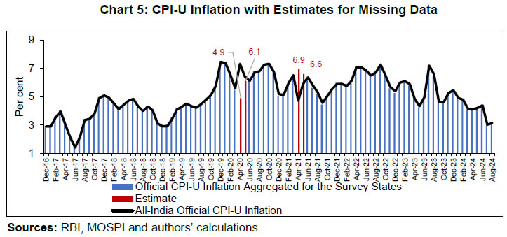
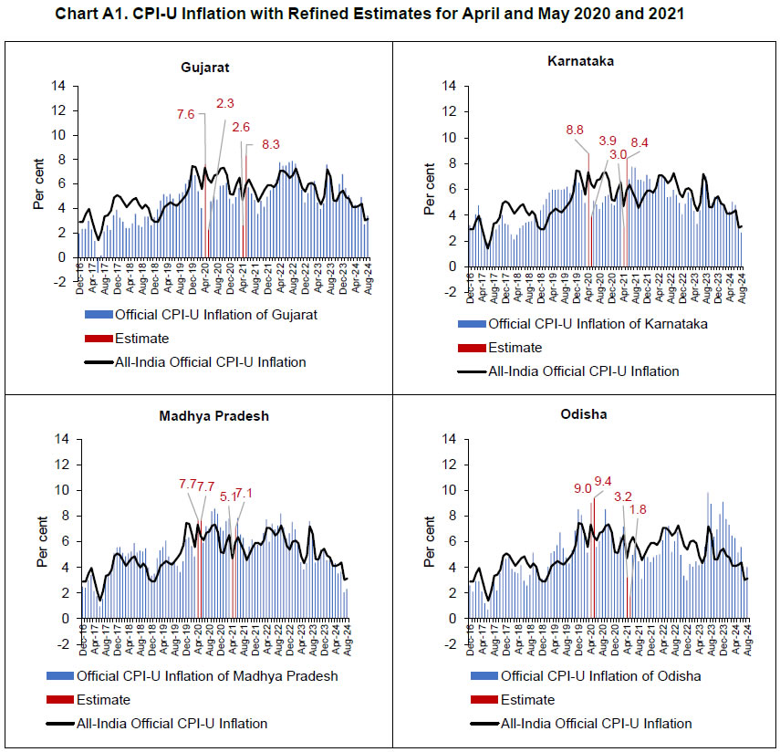
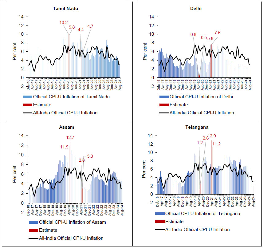
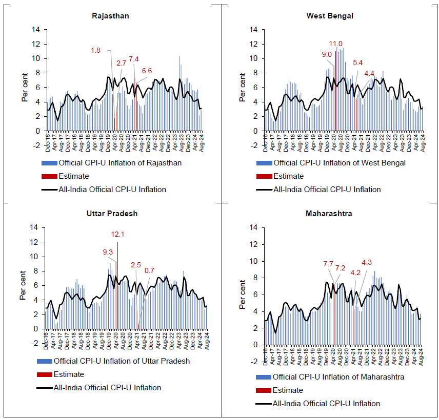
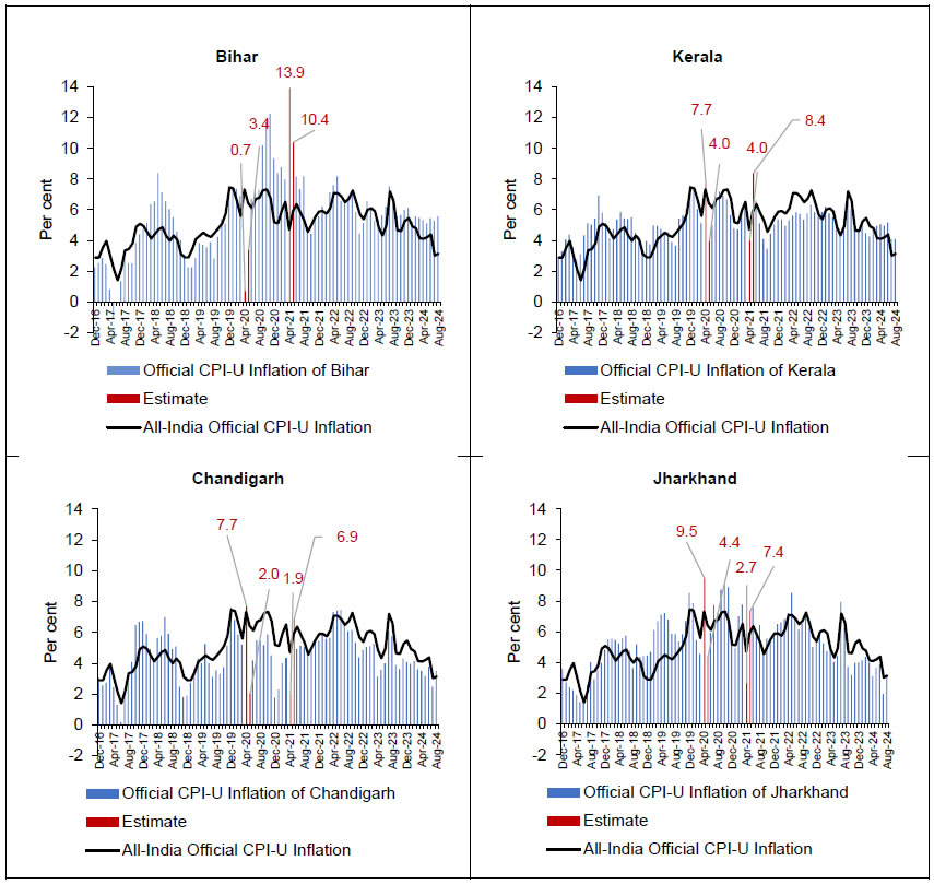
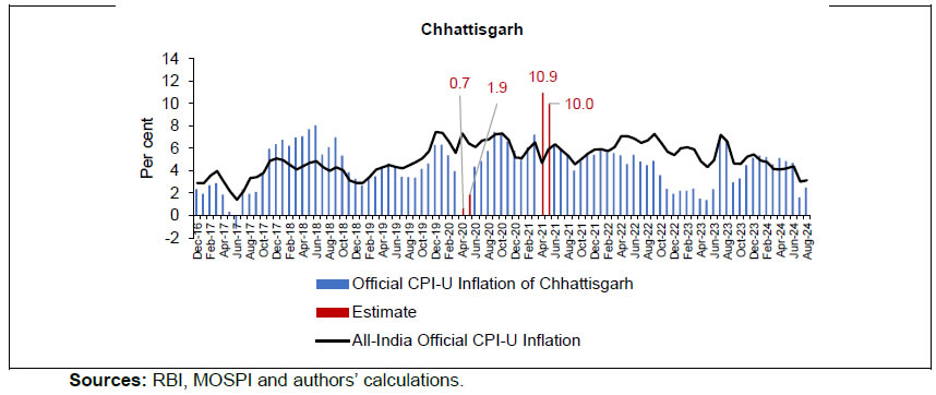
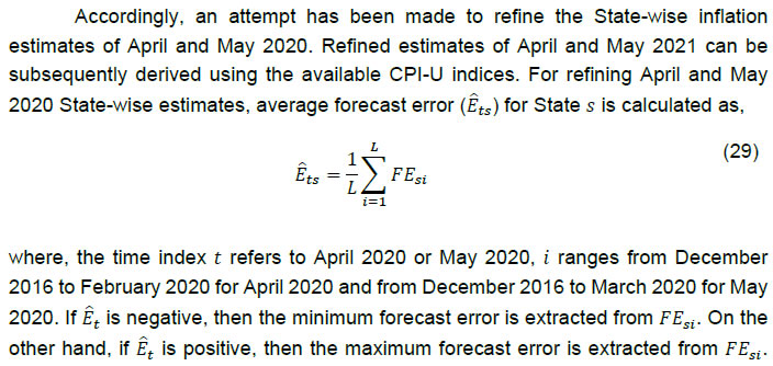 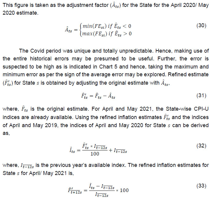 Such refinement of estimates could be made possible only due to the availability of State-wise CPI-U price indices for April and May 2021 and all-India CPI-U inflation for all the four months of April and May 2020 and 2021. The revised estimates for the four months are provided in Annex Tables A3 and A4. State-wise CPI-U inflation figures with refined estimates in the vacant points are plotted in Annex Chart A1. The refined estimates indicate improved performance as they closely follow the all-survey States’ combined CPI-U inflation and the published official all-India inflation (Chart 6). In the light of the low difference between the all-survey states combined inflation and all-India inflation, it may be safe to take the differences between the all-survey centres’ combined CPI-U inflation refined estimates and all-India inflation figures for April and May 2020 and 2021 as the forecast errors which indicates a forecast error in the range of -14 to 13 basis points in the inflation estimates of the missing months (Table 4). 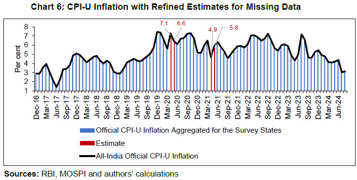
| Table 4: Approximate Forecast Error of the Refined Estimates | | Month | All-India Official CPI-U Inflation | Aggregated State-wise Refined Urban Inflation Estimates | Approximate Error in the Proposed Estimates
(in Basis points) | | April 2020 | 7.330 | 7.111 | -21.708 | | May 2020 | 6.430 | 6.565 | 13.462 | | April 2021 | 4.710 | 4.865 | 15.535 | | May 2021 | 5.910 | 5.766 | -14.364 | | Sources: RBI, MOSPI and authors’ calculations. | Further, to assess the credibility and usefulness of the above exercise, the accuracy of the estimates derived using the proposed method for the post-pandemic period was checked. The error measures of the pre- and post-Covid periods shown in Tables 5 and 6 indicate reduced errors in forecasts in the post-Covid period as compared to the pre-Covid period and this is true not only for the proposed forecasts, but also for the forecasts provided by the professional forecasters. The major improvement in the proposed survey-based forecasts during the post-Covid period is in the case of directional matches. The matches stand at around 65 per cent, which is much higher than those of the professional forecasters (around 39 per cent). The errors of the derived nowcasts and forecasts pertaining to the survey centres are provided in Annex Tables A5 and A6. | Table 5. Performance of Three Months Ahead Forecasts – Pre-Covid Period | | Measure | Proposed | SPF | | RMSE | 1.345 | 1.195 | | MAE | 1.081 | 0.967 | | MAPE | 0.299 | 0.276 | | Correlation | 0.026 | 0.346 | | Directional Matches (in per cent) | 42.105 | 76.923 | | Sources: RBI, MOSPI and authors’ calculations. |
| Table 6. Performance of Three Months Ahead Forecasts – Post Covid Period | | Measure | Proposed | SPF | | RMSE | 1.025 | 0.852 | | MAE | 0.919 | 0.619 | | MAPE | 0.176 | 0.102 | | Correlation | 0.360 | 0.591 | | Directional Matches (in per cent) | 65.217 | 38.889 | | Sources: RBI, MOSPI and authors’ calculations. | As an alternative to the above State-wise inflation estimates, a simple interpolation (simple average of the available neighborhood CPI-U indices) of the CPI-U State-wise indices may also be attempted to derive the State-wise inflation figures for the months using April and May 2020. As two consecutive indices (April and May 2020) are unavailable, simple interpolation will require solving two equations (34) and (35), with two unknowns, i.e., where, CPIUMar−20 and CPIUJun−20 are the CPI-U indices of March and June 2020, respectively, released by MOSPI and the rest two CPIUAar−20 and CPIUMay−20 are unknown. Solving, these equations for each State, result in the estimated State-wise indices of April and May 2020 as given below in equations (36) and (37), As the indices for April and May 2021 are already available, the inflation figures for these months can be accordingly derived (Table 7). | Table 7: Derived CPI-U Inflation for April and May 2020 and 2021 Using Interpolation of Available Indices | | State | Apr-20 | May-20 | Apr-21 | May-21 | | Gujarat | 2.59 | 3.68 | 7.65 | 6.88 | | Karnataka | 2.44 | 3.79 | 9.37 | 8.53 | | Madhya Pradesh | 3.06 | 3.96 | 9.78 | 10.91 | | Odisha | 3.60 | 4.24 | 8.62 | 6.82 | | Tamil Nadu | 3.43 | 4.75 | 11.25 | 9.78 | | Delhi | 0.59 | 0.61 | 5.98 | 7.54 | | Assam | 4.71 | 7.36 | 9.82 | 8.17 | | Telangana | 3.70 | 5.37 | 10.13 | 8.26 | | Rajasthan | 2.66 | 4.03 | 6.42 | 5.24 | | West Bengal | 4.23 | 7.29 | 10.15 | 8.04 | | Uttar Pradesh | 2.67 | 4.48 | 9.15 | 7.96 | | Maharashtra | 2.69 | 4.78 | 9.31 | 6.74 | | Bihar | 3.11 | 4.88 | 11.28 | 8.83 | | Kerala | 2.70 | 3.76 | 9.08 | 8.60 | | Chandigarh | 1.81 | 2.74 | 7.82 | 6.11 | | Jharkhand | 2.61 | 4.36 | 9.56 | 7.41 | | Chhattisgarh | 2.71 | 3.39 | 8.74 | 8.40 | | Combined | 2.83 | 4.41 | 9.18 | 7.89 | | All-India | 5.60 | 5.75 | 6.42 | 6.59 | | Sources: RBI, MOSPI and authors’ calculations. | Using the above State-wise alternative inflation estimates, aggregate inflation estimates and aggregate errors are derived (Table 8). These errors are much higher than the errors shown in Table 4. | Table 8: Error in Interpolated All-India CPI-U Inflation Figures | | | Apr-20 | May-20 | Apr-21 | May-21 | | Derived for All-India Urban Inflation (by interpolation) | 5.60 | 5.75 | 6.42 | 6.59 | | Available for All-India Urban Inflation (Imputed by MOSPI) | 7.33 | 6.43 | 4.71 | 5.91 | | Error in Basis Points | -173.49 | -68.21 | 171.12 | 68.39 | | Sources: RBI, MOSPI and authors’ calculations. | Summing up, the objective was to fill-up the data gaps in the State-wise CPI-U inflation series during the months of April and May 2020 and 2021, owing to the Covid-19 pandemic related restrictions. Using centre-wise urban consumers’ inflation perceptions, three months ahead inflation expectations and past state-wise realised CPI-U inflation figures, State-wise inflation nowcasts and forecasts were calculated, and their performances were studied for a fairly long period. It was found that performance of the proposed State-wise inflation estimates with respect to the published State-wise MOSPI data of CPI-U inflation figures were comparable. Accordingly, the State-wise inflation nowcasts and forecasts were obtained for the months of April and May 2020 and 2021. These estimates were refined using the past error history adjusting for any error in the State-wise estimates due to sudden onset of the pandemic and its grossly unknown cascading impact on inflation. As the forecast error is low compared with alternative estimation forecasts like the interpolation method, the refined estimates provide a better measure to fill the data gaps during the Covid period. V. Conclusion The collection and compilation of official statistics suffered acutely during the outbreak of the Covid-19 pandemic due to the resulting restrictions across the world. In an environment of uncertainty, scarcity of data made it difficult to clearly understand the prevailing economic scenario. To address this issue and to retain the confidence of statisticians and economists in official statistics, statistical organisations attempted to impute the missing data. In India, State-wise CPI indices could not be collected on a full-fledged basis during the pandemic months of April and May 2020. As a result, State-wise CPI inflation figures are unavailable for the months of April and May 2020 and April and May 2021. In this context, this paper uses IESH granular data to derive State-wise CPI-U inflation estimates for these four pandemic months. These State-wise inflation estimates are of critical use in the current inflation targeting regime. Further, these also attempt to resolve the gap in the State-wise inflation series to an extent. When the State-wise inflation estimates are aggregated, the figures closely follow the all-India CPI inflation series published by MOSPI. Accordingly, State-wise inflation estimates for the specific months derived in this paper help in bridging the data gaps. These estimates are expected to be potentially useful for any relevant study. In future, these State-wise inflation estimates may be compared with model-based forecasts. The use of non-parametric methods may also be potentially explored to examine the scope of improvement in the proposed estimates.
@ Purnima Shaw (pshaw@rbi.org.in) is Assistant Adviser and R.K. Sinha is Director in the Department of Statistics and Information Management (DSIM), Reserve Bank of India (RBI). 1 The authors are thankful to Rekha Misra, Binod Bihari Bhoi, Jayaraman Alur Raghavan, Sreeramulu Meruva, Sanjay Singh, Nishant Singh, members of the DSIM Internal Advisory Group, participants of the Department of Economic and Policy Research (DEPR) Study Circle, members of the Development Research Group, the editorial team and an anonymous external reviewer for providing insightful comments which helped in improving the paper. The views and opinions expressed in this paper are those of the authors and do not necessarily represent views of the RBI 2 https://www.ons.gov.uk/economy/inflationandpriceindices/articles/coronavirusandtheeffectsonukprices/2020-05-06 3 https://www.bls.gov/covid19/effects-of-covid-19-pandemic-on-consumer-price-index.htm 4 https://www.abs.gov.au/articles/methods-changes-during-covid-19-period 5 https://www.statssa.gov.za/cpi/documents/CPI_COVID_method_issues_21_05_20.pdf 6 https://www.mospi.gov.in/sites/default/files/press_release/CPI%20Technical%20Note%20on%20Imputation.pdf 7 https://www.mospi.gov.in/sites/default/files/press_release/CPI_PR_120502020.pdf and
https://www.mospi.gov.in/sites/default/files/press_release/CPI_Press%20Release_May%202020.pdf 8 https://www.mospi.gov.in/sites/default/files/press_release/CPI%20Technical%20Note%20on%20Imputation.pdf and
https://mospi.gov.in/press-release/cpi-technical-note-imputation-april-and-may-2020 9 The unit-level data of the survey are present in the Centralised Information Management System of RBI; https://cimsdbie.rbi.org.in/DBIE/#/dbie/home 10 https://www.rbi.org.in/Scripts/BS_PressReleaseDisplay.aspx?prid=49762 11 https://www.rbi.org.in/Scripts/BS_PressReleaseDisplay.aspx?prid=50019 12 https://www.rbi.org.in/Scripts/BS_PressReleaseDisplay.aspx?prid=50275 13 https://www.rbi.org.in/Scripts/BS_PressReleaseDisplay.aspx?prid=50593 14 https://www.rbi.org.in/Scripts/BS_PressReleaseDisplay.aspx?prid=50906 15 https://www.rbi.org.in/Scripts/BS_PressReleaseDisplay.aspx?prid=51492 16 https://www.rbi.org.in/Scripts/BS_PressReleaseDisplay.aspx?prid=51798 17 https://www.rbi.org.in/Scripts/BS_PressReleaseDisplay.aspx?prid=52136 18 The survey, although captures consumers’ inflationary sentiments from select urban centres (mostly State capitals), the sum of the CPI urban weights of the corresponding States stand at 86.8 per cent. Thus, the representation is decent. 19 It has been reported in the literature that the differences in the dynamics of rural and urban inflation in India are transitory and they converge in the long run (Bhoi et al., 2020). 20 Shaw and Sinha (2024) also attempt interpolation. However, here a different approach is presented. 21 The consideration of eight-month window for the official inflation data is indicative. Other numbers instead of eight may be explored. 22 The survey was expanded to urban Jammu from March 2021 round onwards and hence, not considered for the current exercise. 23 The survey centres Mumbai and Nagpur are used in combination to present inflation forecasts for urban Maharashtra. 24 The comparison has been done at aggregated level because SPF does not report the forecasts at the State-level.
References Andridge, R. R., & Little, R. J. A. (2010). A review of Hot Deck Imputation for survey non-response. International Statistical Review, 78, 40-64. Azur, M. J., Stuart, E. A., Frangakis, C., & Leaf, P. J. (2011). Multiple imputation by chained equations: What is it and how does it work? International Journal of Methods in Psychiatric Research, 20(1), 40-49. Bank of Japan. (2020). Impact of COVID-19 on private consumption. Outlook for Economic Activity and Prices, June, 53-56. Beer, B. D., & Tissot, B. (2021). Official statistics in the wake of the Covid-19 pandemic: A central banking perspective. Theoretical Economics Letters, 11, 695-723. Bhoi, B. B., Shekhar, H., & Padhi, I. (2020). Rural-urban inflation dynamics in India. Reserve Bank of India Bulletin, December 2020. Castelletti, B., Delorme, M., Diev, P., Kalantzis, Y., Lalliard A., & Mogliani, M. (2020). Covid-19 and monitoring economic activity: The contribution of high-frequency data. Banque de France EcoNotepad, No. 174. Cavallo, A. (2020). Inflation with Covid consumption baskets. Working Paper 27352, National Bureau of Economic Research. Chapman, J., & Desai, A. (2021). Using payments data to nowcast macroeconomic variables during the onset of Covid-19. Journal of Financial Market Infrastructures, 9, 1-29. https://doi.org/10.21314/JFMI.2021.004 Cheng, S., & Lu, F. (2017). A two-step method for missing spatio-temporal data reconstruction. International Journal of Geo-Information, 6(7), 1-25. Davies, O., Kösem, S., & Whitaker, S. (2020). Predicting Covid-19’s impact on GDP: How can high-frequency data help us? Bank of England, October. Dempster, A. P., Laird, N. M., & Rubin, D. B. (1977). Maximum likelihood from incomplete data via the EM algorithm. Journal of the Royal Statistical Society, Series B (Methodological), 39(1), 1-38. Duma, M., Marwala, T., Twala, B., & Nelwamondo, F. (2013). Partial imputation of unseen records to improve classification using a hybrid multi-layered artificial immune system and genetic algorithm. Applied Soft Computing, 13(12), 4461-4480. Elissavet, R. K. (2017). Missing data in time series and imputation methods. [Unpublished Master's thesis]. University of the Aegean, Samos. Fix, E., & Hodges, J. L. (1951). Discriminatory analysis, nonparametric discrimination: consistency properties. Technical Report 4, USAF School of Aviation Medicine, Randolph Field. Gautier, E., Karadi, P., Amann, J., Conflitti, C., Faber, R., Fabo, B., Fadejeva, L., Fuss, C., Kosma, T., Jouvanceau, V., Martins, F., Menz, J.-O., Messner, T., Petroulas, P., Roldan-Blanco, P., Rumler, F., Sánchez Bachiller, J., Santoro, S., Seward, D., Stanga, I., de Veirman, E., Wieland, E., Wursten, J., & Zimmer, H. (2023). Price adjustment in the Euro area in the low-inflation period: Evidence from consumer and producer micro price data. Occasional Paper Series, No 319, ECB, Frankfurt am Main. Groenwold, R. H. H., White, I. R., Donders, A. R. T., Carpenter, J. R., Altman, D. G., & Moons, K. G. M. (2012). Missing covariate data in clinical research: When and when not to use the missing-indicator method for analysis. Canadian Medical Association Journal, 184(11), 1265-1269. Hinge, D. (2020). Covid-19 policy-making and the need for high-speed data. Central Banking, August. https://www.centralbanking.com/central-banks/economics/data/7668551/covid-19-policy-making-and-the-need-for-high-speed-data Holt, C. E. (1957). Forecasting trends and seasonals by exponentially weighted moving averages. ONR Memorandum, 52, Carnegie Institute of Technology, Pittsburg, USA. Hopkins, A., & Sherman, M. (2020). How has the COVID-19 pandemic affected daily spending patterns? Central Bank of Ireland, April. https://www.centralbank.ie/statistics/statistical-publications/behind-the-data/how-has-the-covid-19-pandemic-affected-daily-spending-patterns Huynh, K., Lao, H., Sabourin, P., & Welte, A. (2020). What do high-frequency expenditure network data reveal about spending and inflation during COVID‑19? Staff Analytical Note 2020-20. Bank of Canada. INSEE (2020). High-frequency data are especially useful for economic forecasting in periods of devastating crisis. Point de Conjoncture, 17 June, 29-34. Jonckheere, J., & Zimmer, H. (2020). Consumer prices in light of the COVID-19 crisis. Economic Review, Nationale Bank Van België/Banque Nationale de Belgique, December. Kálmán, R. E. (1960), A new approach to linear filtering and prediction problems. Journal of Basic Engineering, 82, 35-45. Kálmán, R. E., & Bucy, R. S. (1961). New results in linear filtering and prediction theory. Journal of Basic Engineering, 83, 95-108. Kim, Y. J., & Chi, M. (2018). Temporal belief memory: Imputing missing data during RNN training”. Proceedings of the Twenty-Seventh International Joint Conference on Artificial Intelligence. Kouvavas, O., Trezzi, R., Eiglsperger, M., Goldhammer, B., & Gonçalves, E. (2020). Consumption patterns and inflation measurement issues during the COVID19 pandemic. Economic Bulletin, 7, ECB, Frankfurt am Main. Kuhn, M., & Johnson, K. (2020). Feature Engineering and Selection: A Practical Approach for Predictive Models. CRC Press, Boca Raton. Molnar, F. J., Hutton, B., & Fergusson, D. (2008). Does analysis using “last observation carried forward” introduce bias in dementia research? Canadian Median Association Journal, 179(8), 751-753. Patterson, J., & Gibson, A. (2017). Deep Learning: A Practitioner’s Approach. O’Reilly Media, Sebastopol. Pratama, I., Parmanasari, A. E., & Indrayani, R. (2016). A review of missing values handling methods on time-series data. International Conference on Information Technology and Innovation (ICITSI), 2016. Ribeiro, S. M., & Castro, C. L. D. (2022). Missing data in time series: A review of imputation methods and case study. Learning and Nonlinear Models. Journal of the Brazilian Society on Computational Intelligence, 20(1), 31-46. Rocha, J., Oliveira, S., & Viana, C. (2024). Time Series Analysis - Recent Advances, New Perspectives and Applications. IntechOpen, United Kingdom. Sharma, N. K., & M. Bicchal. (2018). The properties of inflation expectations: Evidence for India. Economia, 19(1), 74–89. https://doi.org/10.1016/j.econ.2017.12.002. Shaw, P. (2019). Using rational expectations to predict inflation. Reserve Bank of India Occasional Papers, 40(1), 85–104. Shaw, P. (2024). Reading consumers’ minds: An analysis of inflation expectations. Macroeconomics and Finance in Emerging Market Economies. https://doi.org/10.1080/17520843.2024.2352955. Shaw, P., & Sinha, R. K. (2024). State-level inflation forecasts for India: Based on data from Inflation Expectations Survey of Households. Reserve Bank of India Working Paper Series, WPS (DEPR): 09/2024. Singh, D. P., Mishra, A., & Shaw, P. (2024). Taking cognisance of households’ inflation expectations in India. Macroeconomics and Finance in Emerging Market Economies. https://doi.org/10.1080/17520843.2024.2350250. Sinha, R. K. (2023). Inflation and inflation expectations: A distributional mapping. Reserve Bank of India Bulletin, September 2023. Swerling, P. (1958). First-order error propagation in a stagewise smoothing procedure for satellite observations, CA: RAND Corporation, Santa Monica. Yoon, J., Jordon, J., & Schaar, M. V. D. (2018). GAIN: Missing data imputation using generative adversarial nets. In J. Dy & A. Krause (Ed.), Proceedings of the 35th International Conference on Machine Learning: Vol 80, 5689–5698, Stockholm Sweden, 10–15 Jul 2018, PMLR.
Annex | Table A1. Estimated CPI-U Inflation for April and May, 2020 | | State | Actual | Estimated | Actual | | Feb-20 | Mar-20 | Apr-20 | May-20 | Jun-20 | Jul-20 | | Gujarat | 5.410 | 4.020 | 5.232 | 6.383 | 4.590 | 4.990 | | Karnataka | 5.950 | 4.960 | 6.300 | 6.300 | 5.120 | 4.830 | | Madhya Pradesh | 5.660 | 4.840 | 4.440 | 4.914 | 5.940 | 7.200 | | Odisha | 6.970 | 5.160 | 5.648 | 6.893 | 5.600 | 6.050 | | Tamil Nadu | 7.530 | 6.500 | 5.227 | 6.528 | 6.320 | 7.300 | | Delhi | 3.320 | 2.890 | 3.341 | 2.943 | 1.690 | 3.670 | | Assam | 9.220 | 8.430 | 8.106 | 9.120 | 10.100 | 10.930 | | Telangana | 8.270 | 7.370 | 5.449 | 7.229 | 7.370 | 7.880 | | Rajasthan | 6.510 | 5.040 | 4.546 | 5.345 | 5.230 | 5.310 | | West Bengal | 8.410 | 6.440 | 3.893 | 6.672 | 11.640 | 10.950 | | Uttar Pradesh | 8.200 | 7.360 | 4.334 | 7.342 | 5.890 | 6.380 | | Maharashtra | 5.790 | 5.030 | 5.077 | 5.820 | 6.390 | 7.340 | | Bihar | 7.360 | 6.910 | 4.907 | 7.076 | 6.710 | 7.460 | | Kerala | 6.040 | 5.120 | 4.619 | 6.153 | 5.000 | 6.660 | | Chandigarh | 5.850 | 5.220 | 3.943 | 5.864 | 4.180 | 5.480 | | Jharkhand | 5.460 | 4.560 | 6.780 | 6.698 | 5.940 | 7.760 | | Chhattisgarh | 5.380 | 3.970 | 4.458 | 5.345 | 4.340 | 4.860 | | Combined | 6.511 | 5.495 | 4.901 | 6.125 | 6.117 | 6.784 | | Sources: RBI, MOSPI and authors’ calculations. |
| Table A2. Estimated CPI-U Inflation for April and May, 2021 | | State | Actual | Estimated | Actual | | Feb-21 | Mar-21 | Apr-21 | May-21 | Jun-21 | Jul-21 | | Gujarat | 4.920 | 5.660 | 5.062 | 5.641 | 5.710 | 5.230 | | Karnataka | 5.870 | 6.730 | 5.208 | 5.470 | 6.770 | 7.770 | | Madhya Pradesh | 7.600 | 7.800 | 7.413 | 8.256 | 7.850 | 6.580 | | Odisha | 6.380 | 7.180 | 6.640 | 6.873 | 4.970 | 5.700 | | Tamil Nadu | 8.050 | 8.470 | 7.254 | 7.966 | 8.310 | 6.930 | | Delhi | 3.010 | 3.560 | 3.809 | 3.505 | 6.940 | 5.280 | | Assam | 6.180 | 5.780 | 9.833 | 7.576 | 4.590 | 3.370 | | Telangana | 6.180 | 7.260 | 7.923 | 7.963 | 5.960 | 6.090 | | Rajasthan | 3.560 | 4.330 | 5.355 | 4.695 | 4.110 | 3.600 | | West Bengal | 7.220 | 7.650 | 11.181 | 9.336 | 5.060 | 5.760 | | Uttar Pradesh | 4.320 | 4.790 | 6.552 | 4.785 | 5.960 | 5.740 | | Maharashtra | 6.100 | 6.830 | 7.213 | 6.742 | 5.870 | 4.560 | | Bihar | 8.770 | 7.960 | 10.098 | 10.003 | 8.160 | 7.340 | | Kerala | 5.890 | 6.360 | 6.658 | 6.580 | 6.600 | 5.120 | | Chandigarh | 3.990 | 4.330 | 5.397 | 4.376 | 4.920 | 5.130 | | Jharkhand | 7.010 | 7.770 | 8.917 | 8.998 | 7.590 | 5.920 | | Chhattisgarh | 6.070 | 7.220 | 6.763 | 7.292 | 6.380 | 5.890 | | Combined | 5.893 | 6.489 | 6.942 | 6.605 | 6.286 | 5.638 | | Sources: RBI, MOSPI and authors’ calculations. |
| Table A3. Estimated CPI-U Inflation for April and May, 2020 - Refined | | State | Actual | Refined Estimate | Actual | | Feb-20 | Mar-20 | Apr-20 | May-20 | Jun-20 | Jul-20 | | Gujarat | 5.410 | 4.020 | 7.617 | 2.283 | 4.590 | 4.990 | | Karnataka | 5.950 | 4.960 | 8.764 | 3.912 | 5.120 | 4.830 | | Madhya Pradesh | 5.660 | 4.840 | 7.666 | 7.669 | 5.940 | 7.200 | | Odisha | 6.970 | 5.160 | 9.024 | 9.426 | 5.600 | 6.050 | | Tamil Nadu | 7.530 | 6.500 | 10.193 | 9.814 | 6.320 | 7.300 | | Delhi | 3.320 | 2.890 | 0.754 | 0.536 | 1.690 | 3.670 | | Assam | 9.220 | 8.430 | 11.903 | 12.691 | 10.100 | 10.930 | | Telangana | 8.270 | 7.370 | 1.167 | 2.559 | 7.370 | 7.880 | | Rajasthan | 6.510 | 5.040 | 1.757 | 2.684 | 5.230 | 5.310 | | West Bengal | 8.410 | 6.440 | 8.952 | 11.024 | 11.640 | 10.950 | | Uttar Pradesh | 8.200 | 7.360 | 9.293 | 12.052 | 5.890 | 6.380 | | Maharashtra | 5.790 | 5.030 | 7.736 | 7.230 | 6.390 | 7.340 | | Bihar | 7.360 | 6.910 | 0.725 | 3.385 | 6.710 | 7.460 | | Kerala | 6.040 | 5.120 | 7.731 | 3.951 | 5.000 | 6.660 | | Chandigarh | 5.850 | 5.220 | 7.702 | 2.023 | 4.180 | 5.480 | | Jharkhand | 5.460 | 4.560 | 9.495 | 4.398 | 5.940 | 7.760 | | Chhattisgarh | 5.380 | 3.970 | 0.668 | 1.870 | 4.340 | 4.860 | | Combined | 6.511 | 5.495 | 7.113 | 6.565 | 6.117 | 6.784 | | Sources: RBI, MOSPI and authors’ calculations. |
| Table A4. Estimated CPI-U Inflation for April and May 2021 - Refined | | State | Actual | Refined Estimate | Actual | | Feb-21 | Mar-21 | Apr-21 | May-21 | Jun-21 | Jul-21 | | Gujarat | 4.920 | 5.660 | 2.627 | 8.336 | 5.710 | 5.230 | | Karnataka | 5.870 | 6.730 | 3.010 | 8.402 | 6.770 | 7.770 | | Madhya Pradesh | 7.600 | 7.800 | 5.080 | 7.092 | 7.850 | 6.580 | | Odisha | 6.380 | 7.180 | 3.213 | 1.757 | 4.970 | 5.700 | | Tamil Nadu | 8.050 | 8.470 | 4.431 | 4.713 | 8.310 | 6.930 | | Delhi | 3.010 | 3.560 | 5.803 | 7.616 | 6.940 | 5.280 | | Assam | 6.180 | 5.780 | 2.767 | 3.047 | 4.590 | 3.370 | | Telangana | 6.180 | 7.260 | 12.887 | 11.220 | 5.960 | 6.090 | | Rajasthan | 3.560 | 4.330 | 7.371 | 6.619 | 4.110 | 3.600 | | West Bengal | 7.220 | 7.650 | 5.376 | 4.409 | 5.060 | 5.760 | | Uttar Pradesh | 4.320 | 4.790 | 2.537 | 0.660 | 5.960 | 5.740 | | Maharashtra | 6.100 | 6.830 | 4.184 | 4.301 | 5.870 | 4.560 | | Bihar | 8.770 | 7.960 | 13.914 | 10.405 | 8.160 | 7.340 | | Kerala | 5.890 | 6.360 | 3.995 | 8.393 | 6.600 | 5.120 | | Chandigarh | 3.990 | 4.330 | 1.926 | 6.851 | 4.920 | 5.130 | | Jharkhand | 7.010 | 7.770 | 2.672 | 7.365 | 7.590 | 5.920 | | Chhattisgarh | 6.070 | 7.220 | 10.948 | 10.011 | 6.380 | 5.890 | | Combined | 5.893 | 6.489 | 4.865 | 5.766 | 6.286 | 5.638 | | Sources: RBI, MOSPI and authors’ calculations. |
| Table A5: Forecasts' Errors – Pre-Covid Period | | Nowcasts | RMSE | | Gujarat | 1.462 | Delhi | 1.095 | Uttar Pradesh | 2.069 | Jharkhand | 1.321 | | Karnataka | 1.133 | Assam | 1.346 | Maharashtra | 0.838 | Chhattisgarh | 2.037 | | Madhya Pradesh | 1.333 | Telangana | 2.366 | Bihar | 2.151 | | | | Odisha | 1.391 | Rajasthan | 1.415 | Kerala | 1.124 | | | | Tamil Nadu | 1.569 | West Bengal | 2.062 | Chandigarh | 2.065 | | | | All Centres Combined - 1.164 | | MAE | | Gujarat | 1.113 | Delhi | 0.902 | Uttar Pradesh | 1.676 | Jharkhand | 1.136 | | Karnataka | 0.929 | Assam | 1.133 | Maharashtra | 0.687 | Chhattisgarh | 1.620 | | Madhya Pradesh | 1.128 | Telangana | 1.873 | Bihar | 1.838 | | | | Odisha | 1.150 | Rajasthan | 1.110 | Kerala | 0.937 | | | | Tamil Nadu | 1.370 | West Bengal | 1.605 | Chandigarh | 1.646 | | | | All Centres Combined - 0.920 | | MAPE | | Gujarat | 0.451 | Delhi | 0.262 | Uttar Pradesh | 0.553 | Jharkhand | 0.348 | | Karnataka | 0.273 | Assam | 0.274 | Maharashtra | 0.213 | Chhattisgarh | 0.782 | | Madhya Pradesh | 0.355 | Telangana | 0.763 | Bihar | 2.248 | | | | Odisha | 0.413 | Rajasthan | 0.329 | Kerala | 0.213 | | | | Tamil Nadu | 0.400 | West Bengal | 0.449 | Chandigarh | 1.341 | | | | All Centres Combined - 0.280 | | Three Months Ahead Forecasts | RMSE | | Gujarat | 1.571 | Delhi | 1.343 | Uttar Pradesh | 2.649 | Jharkhand | 1.686 | | Karnataka | 1.436 | Assam | 2.078 | Maharashtra | 1.068 | Chhattisgarh | 2.628 | | Madhya Pradesh | 1.395 | Telangana | 2.443 | Bihar | 2.473 | | | | Odisha | 1.573 | Rajasthan | 1.520 | Kerala | 1.223 | | | | Tamil Nadu | 2.004 | West Bengal | 2.919 | Chandigarh | 1.904 | | | | All Centres Combined - 1.345 | | MAE | | Gujarat | 1.239 | Delhi | 1.142 | Uttar Pradesh | 2.201 | Jharkhand | 1.485 | | Karnataka | 1.171 | Assam | 1.793 | Maharashtra | 0.832 | Chhattisgarh | 2.133 | | Madhya Pradesh | 1.053 | Telangana | 2.088 | Bihar | 2.174 | | | | Odisha | 1.285 | Rajasthan | 1.237 | Kerala | 0.951 | | | | Tamil Nadu | 1.670 | West Bengal | 2.383 | Chandigarh | 1.507 | | | | All Centres Combined - 1.081 | | MAPE | | Gujarat | 0.452 | Delhi | 0.331 | Uttar Pradesh | 0.642 | Jharkhand | 0.395 | | Karnataka | 0.337 | Assam | 0.398 | Maharashtra | 0.238 | Chhattisgarh | 0.630 | | Madhya Pradesh | 0.339 | Telangana | 0.716 | Bihar | 2.275 | | | | Odisha | 0.411 | Rajasthan | 0.343 | Kerala | 0.200 | | | | Tamil Nadu | 0.427 | West Bengal | 0.630 | Chandigarh | 1.347 | | | | All Centres Combined - 0.299 | | Sources: RBI, MOSPI and authors’ calculations. |
| Table A6: Forecasts' Errors – Post-Covid Period | | Nowcasts | RMSE | | Gujarat | 1.446 | Delhi | 1.365 | Uttar Pradesh | 1.175 | Jharkhand | 1.628 | | Karnataka | 1.044 | Assam | 1.777 | Maharashtra | 1.267 | Chhattisgarh | 1.657 | | Madhya Pradesh | 1.333 | Telangana | 1.200 | Bihar | 1.856 | | | | Odisha | 1.886 | Rajasthan | 1.551 | Kerala | 0.988 | | | | Tamil Nadu | 1.364 | West Bengal | 1.850 | Chandigarh | 1.074 | | | | All Centres Combined - 0.978 | | MAE | | Gujarat | 1.246 | Delhi | 1.041 | Uttar Pradesh | 0.945 | Jharkhand | 1.326 | | Karnataka | 0.746 | Assam | 1.329 | Maharashtra | 1.061 | Chhattisgarh | 1.259 | | Madhya Pradesh | 1.112 | Telangana | 0.840 | Bihar | 1.458 | | | | Odisha | 1.406 | Rajasthan | 1.267 | Kerala | 0.714 | | | | Tamil Nadu | 1.138 | West Bengal | 1.548 | Chandigarh | 0.811 | | | | All Centres Combined - 0.780 | | MAPE | | Gujarat | 0.244 | Delhi | 0.359 | Uttar Pradesh | 0.189 | Jharkhand | 0.250 | | Karnataka | 0.139 | Assam | 0.298 | Maharashtra | 0.197 | Chhattisgarh | 0.329 | | Madhya Pradesh | 0.196 | Telangana | 0.130 | Bihar | 0.217 | | | | Odisha | 0.248 | Rajasthan | 0.244 | Kerala | 0.149 | | | | Tamil Nadu | 0.207 | West Bengal | 0.295 | Chandigarh | 0.204 | | | | All Centres Combined - 0.149 | | Three Months Ahead Forecasts | RMSE | | Gujarat | 1.528 | Delhi | 1.734 | Uttar Pradesh | 1.241 | Jharkhand | 1.345 | | Karnataka | 1.164 | Assam | 2.294 | Maharashtra | 1.595 | Chhattisgarh | 1.940 | | Madhya Pradesh | 1.534 | Telangana | 1.700 | Bihar | 1.773 | | | | Odisha | 2.062 | Rajasthan | 1.766 | Kerala | 0.879 | | | | Tamil Nadu | 1.363 | West Bengal | 2.871 | Chandigarh | 1.343 | | | | All Centres Combined - 1.025 | | MAE | | Gujarat | 1.221 | Delhi | 1.322 | Uttar Pradesh | 1.043 | Jharkhand | 1.170 | | Karnataka | 0.936 | Assam | 1.869 | Maharashtra | 1.387 | Chhattisgarh | 1.563 | | Madhya Pradesh | 1.271 | Telangana | 1.400 | Bihar | 1.353 | | | | Odisha | 1.599 | Rajasthan | 1.454 | Kerala | 0.751 | | | | Tamil Nadu | 1.120 | West Bengal | 2.278 | Chandigarh | 1.017 | | | | All Centres Combined - 0.919 | | MAPE | | Gujarat | 0.238 | Delhi | 0.420 | Uttar Pradesh | 0.202 | Jharkhand | 0.228 | | Karnataka | 0.190 | Assam | 0.430 | Maharashtra | 0.247 | Chhattisgarh | 0.459 | | Madhya Pradesh | 0.245 | Telangana | 0.277 | Bihar | 0.209 | | | | Odisha | 0.292 | Rajasthan | 0.290 | Kerala | 0.148 | | | | Tamil Nadu | 0.220 | West Bengal | 0.378 | Chandigarh | 0.274 | | | | All Centres Combined - 0.176 | | Sources: RBI, MOSPI and authors’ calculations. |
     |